8 RootLocus Analysis 8 1 Determining stability bonds

8. Root-Locus Analysis 8. 1 Determining stability bonds in closed-loop systems DEU-MEE 5017 Advanced Automatic Control

Example 8. 1: Examine the closed-loop stability by using pzmap() function in MATLAB: np=1; dp=[1, 3, 5, 2]; gp=tf(np, dp); pzmap(gp); hold on; %return for K = 2: 2: 30 nh=K; dh=[1 3 5 2+K]; h=tf(nh, dh); pzmap(h); end;

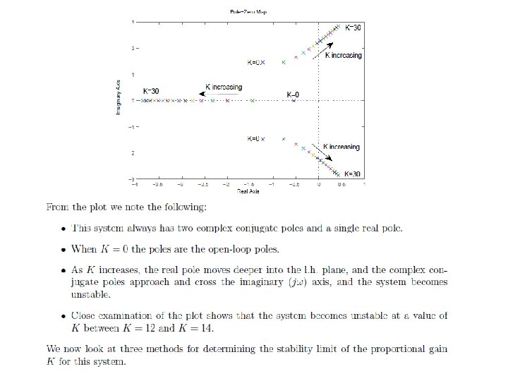
Example 8. 2: Consider Example 8. 1. Find the range of K for which the considered system will be stable. Routh array: MATLAB: K = 13; nh=K; dh=[1 3 5 2+K]; h=tf(nh, dh); pzmap(h); >>p=roots(dh) p= -3. 0000 0. 0000 + 2. 2361 i 0. 0000 - 2. 2361 i

8. 3 Root-Locus Method We hae seen that the closed-loop poles change as controller parameters vary. A root-locus is an s-plane plot of the paths that the closed-loop poles as a controller parameter varies. Let’s start with an example. K: Control gain R(s) Properties and construction of the Root Loci: Rule-1. The K=0 points on the root loci are at the poles of KG p(s). >> dp=[1, 11, 48, 104, 96, 0]; roots(dp) Rule-2. The K= ± points on the rooy loci are at the zeros of KGp(s). >> np=[1, 1]; roots(np) Tekstil Mühendisliği-MAK 3026 Kontrol Sitemleri Doç. Dr. Levent Malgaca, 2015 Bahar

Rule-3. The number of branches of the root loci is equal to the order of D p(s). n= The order of Dp(s): 5, so, there are 5 branches of the root loci. Rule-4. The root-loci are symmetrical with respect to the real axis. Rule-5. The properties of the root loci near infinity in the s-plane are described by the asymptotes. For large values of s, the root loci for K 0 are asymptotic to asymptotes with angles given by n m n : The order of Dp(s) m : The order of Np(s) For number of n–m asymptotes: for k= 0, 1, 2, 3 Rule-6. The intersect of the asymptotes of the root loci lies on the real axis of the splane.

Rules 7 -8. Angles of departure and angles arrival (Kuo: Page, 485). We will not cover these rules. At this stage, we will use “rlocus()” command in MATLAB to obtain a rootlocus plot. We will do analyses and syntheses from the plot by using the properties of the root-locus method. MATLAB : np=[1, 1]; dp=[1, 11, 48, 104, 96, 0] rlocus(np, dp)

Rule-9. Intersection of the Root Loci with the imaginary axis. a) We can use the Routh-Hurwitz method. Routh array: From the first column of array: or >>K=190. 2; dh=[1, 11, 48, 104, 96+K, K]; p=roots(dh) -5. 0806 ± 2. 5862 i ± 2. 6413 i (The coordinate of the point A) -0. 8389

b) We can use MATLAB : np=[1, 1]; dp=[1, 11, 48, 104, 96, 0]; rlocus(np, dp) rlocfind(np, dp) Select the point A MATLAB gives the results for the selected point: and ± 2. 6413 i A

b) We can use the property that the pole s=i at A must satisfy the characteristic equation when the value of K at A is known. K=190. 2 (at A) s=i

Rule-10. Breekaway points on the root loci of an equation correspond to multipleorder roots of the equation. The breakaway points on the root loci of Dh=0 must satisfy >>d=[4, 38, 140, 248, 208, 96]; roots(d) -3. 5462 -2. 4226 + 1. 3263 i -2. 4226 - 1. 3263 i -0. 5543 + 0. 7616 i -0. 5543 - 0. 7616 i

8. 1 Design with the Root-Locus Method Remember that we can calculate the system dynamic parameters from the eigenvalues. S-plane ωn Im iω φ -σ Re At design stage, we can determine the value of controller gain K so that the closed-loop system has the desired damping ratio and natural frequency. Example 8. 3: Determine the controller gain of K so that the closed-loop system has. MATLAB : ksi=0. 341; wn=5; np=[1, 1]; dp=[1, 11, 48, 104, 96, 0]; rlocus(np, dp) sgrid([ksi/2 ksi 2. 5*ksi], [wn/2 wn]) rlocfind(np, dp) For 2 nd order prototype transfer function

Example 8. 3: (Continue) Analyze the eigenvalues and the step response of the closed-loop system for the determined K. MATLAB : k=66. 6; p=rlocus(gp, k) h=feedback(k*gp, 1) step(h) p =-4. 4559 ± 1. 9242 i -0. 7596 ± 2. 0955 i -0. 5690 H(s) =