8 Measurement Errors 1 Objectives List some sources

(8) Measurement Errors 1

Objectives • List some sources of measurement errors. • Classify measurement errors into systematic and random errors. • Study some statistical tools to treat measurement data contaminated by random errors. 2

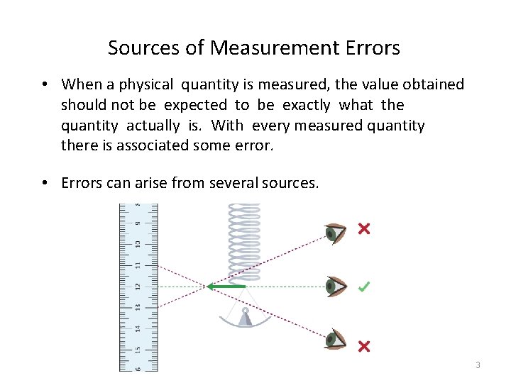
Sources of Measurement Errors • When a physical quantity is measured, the value obtained should not be expected to be exactly what the quantity actually is. With every measured quantity there is associated some error. • Errors can arise from several sources. 3

Sources of Measurement Errors (1) Instrument errors: occur in the manufacturing of instrument or due to the use of instrument under different conditions (e. g. temperature) to which it was calibrated. (2) Human errors: wrong reading of an instrument. (3) Insertion errors: the measuring device affects the measured quantity (loading effect) (4) Errors of unexplainable origin: classified as random errors. 4

Types of Measurement Errors • Measurement errors can be classified into random or systematic. • Systematic errors do not vary from one reading to another (instrument, human, and insertion errors). • Random errors, on the contrary, are caused by unpredictable variations in the measurement system. 5

Random Errors • Random errors are usually observed as small perturbations of repeated measurements around the correct value, i. e. positive and negative errors occur in approximately equal numbers for repeated measurements made of the same constant quantity. • Random errors can largely be eliminated by calculating the average or mean of a number of repeated measurements. • In the next slides, an introduction to statistics is provided. It contains a description of how to discuss and report measurements that have some randomness associated with them. 6

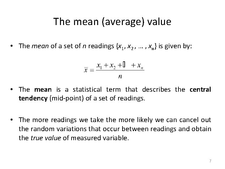
The mean (average) value • The mean of a set of n readings {x 1, x 2 , … , xn} is given by: • The mean is a statistical term that describes the central tendency (mid-point) of a set of readings. • The more readings we take the more likely we cancel out the random variations that occur between readings and obtain the true value of measured variable. 7

Example 1 • The following are five measurements of the length of a steel bar (in mm): {407, 403, 404, 403, 408}. The mean of the readings is 405 mm. • Imagine that a 6 th reading of 441 mm was obtained. The mean of the 6 readings is 411 mm. • The two mean values are quite different. • The reason is that the 441 mm reading is much higher than the other readings. This reading is called an outlier. Outlier is too low or high reading compared to the rest of readings. • Therefore, the mean is very sensitive to outliers. 8

The median • The median is another statistical term which plays a role similar to the mean in describing the central tendency of a set of readings. • Median is less sensitive to outliers. Therefore, it is sometimes taken as a better measure of the mid point. • To calculate the median, we do not sum the measurements, but we write them in an ascending order. 9

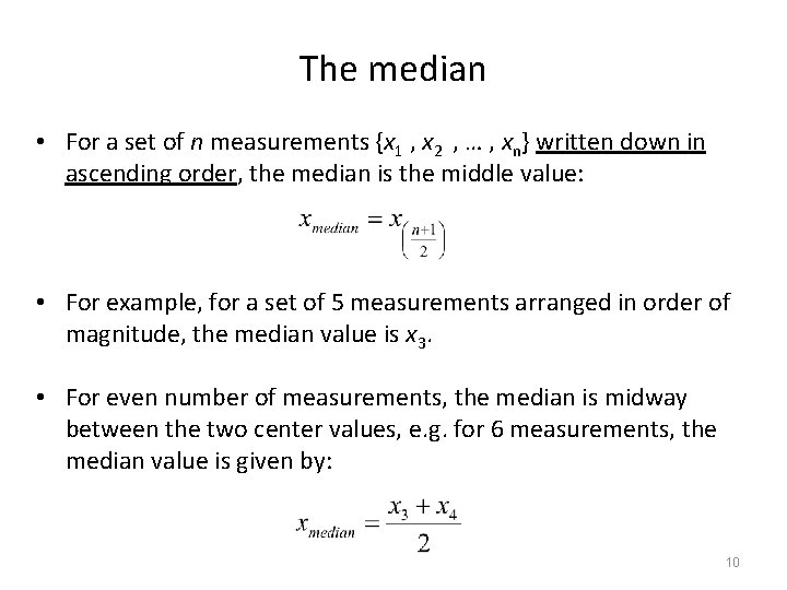
The median • For a set of n measurements {x 1 , x 2 , … , xn} written down in ascending order, the median is the middle value: • For example, for a set of 5 measurements arranged in order of magnitude, the median value is x 3. • For even number of measurements, the median is midway between the two center values, e. g. for 6 measurements, the median value is given by: 10

Example 2 • Back to Example 1, recall that mean of the set of 5 measurements, {407, 403, 404, 403, 408}, is 405 mm. • To calculate the median, we reorder the readings as {403, 404, 407, 408}. The median is 404 mm. • With 6 readings, {407, 403, 404, 403, 408, 441}, the mean is 411 mm. The median is (404 + 407)/2 = 405. 5 mm. • We realize that the median does not change too much compared to the mean. 11

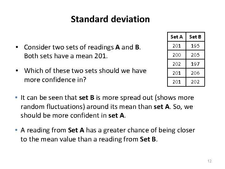
Standard deviation • Consider two sets of readings A and B. Both sets have a mean 201. • Which of these two sets should we have more confidence in? Set A Set B 201 195 200 205 202 197 201 206 201 202 • It can be seen that set B is more spread out (shows more random fluctuations) around its mean than set A. So, we should be more confident in set A. • A reading from Set A has a greater chance of being closer to the mean value than a reading from Set B. 12

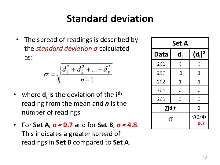
Standard deviation • The spread of readings is described by the standard deviation σ calculated as: ith • where di is the deviation of the reading from the mean and n is the number of readings. • For Set A, σ = 0. 7 and for Set B, σ = 4. 8. This indicates a greater spread of readings in Set B compared to Set A Data di (di)2 201 0 0 200 -1 1 202 1 1 201 0 0 ∑(di)2 2 σ √(2/4) = 0. 7 13

Graphical data analysis • Graphs are very useful in analyzing how random measurement errors are distributed. A commonly used graph for this purpose is the histogram. • To draw the histogram, bands of equal width across the range of measurement values are defined and the number of measurements within each band is counted. • For example, the histogram of the following set of 23 readings: {407, 404, 405, 407, 402, 406, 409, 408, 405, 406, 410, 406, 408, 406, 409, 406, 405, 409, 406, 407}, using bands 2 mm wide, is shown next. 14

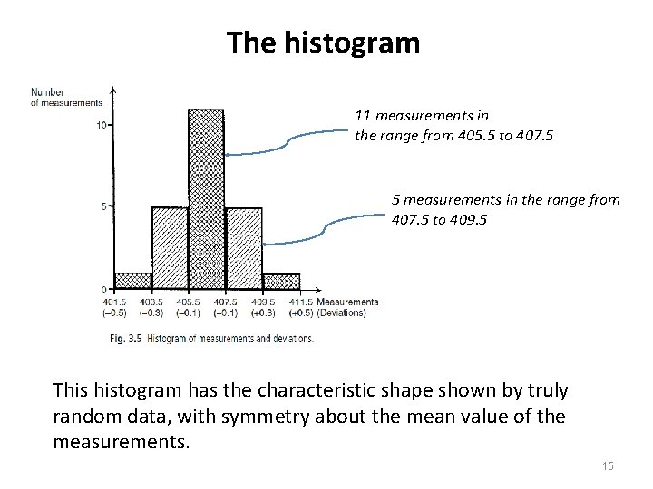
The histogram 11 measurements in the range from 405. 5 to 407. 5 5 measurements in the range from 407. 5 to 409. 5 This histogram has the characteristic shape shown by truly random data, with symmetry about the mean value of the measurements. 15

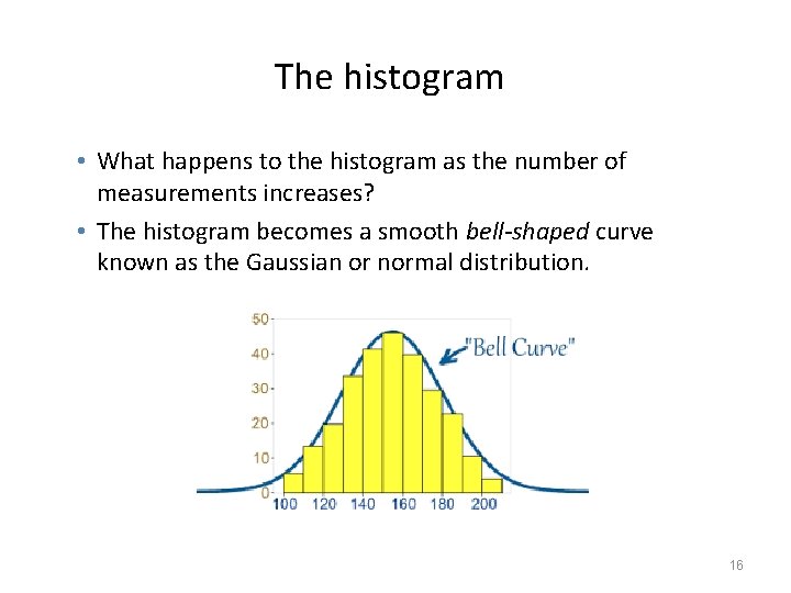
The histogram • What happens to the histogram as the number of measurements increases? • The histogram becomes a smooth bell-shaped curve known as the Gaussian or normal distribution. 16

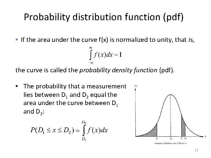
Probability distribution function (pdf) • If the area under the curve f(x) is normalized to unity, that is, the curve is called the probability density function (pdf). • The probability that a measurement lies between D 1 and D 2 equal the area under the curve between D 1 and D 2: 17

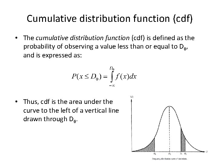
Cumulative distribution function (cdf) • The cumulative distribution function (cdf) is defined as the probability of observing a value less than or equal to D 0, and is expressed as: • Thus, cdf is the area under the curve to the left of a vertical line drawn through D 0. 18

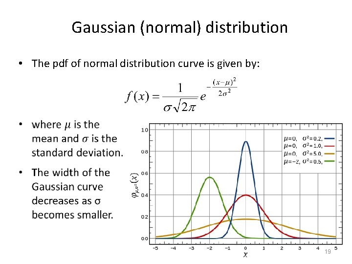
Gaussian (normal) distribution • The pdf of normal distribution curve is given by: 19

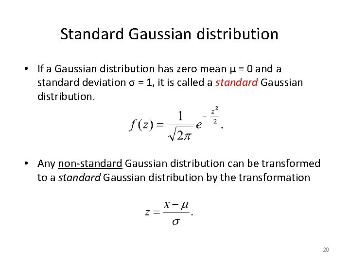
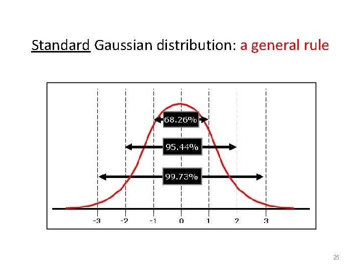
Standard Gaussian distribution • If a Gaussian distribution has zero mean μ = 0 and a standard deviation σ = 1, it is called a standard Gaussian distribution. • Any non-standard Gaussian distribution can be transformed to a standard Gaussian distribution by the transformation 20

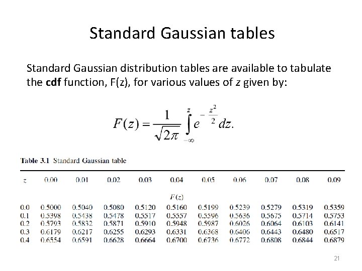
Standard Gaussian tables Standard Gaussian distribution tables are available to tabulate the cdf function, F(z), for various values of z given by: 21

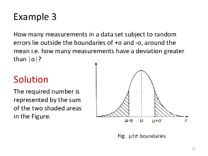
Example 3 How many measurements in a data set subject to random errors lie outside the boundaries of +σ and -σ, around the mean i. e. how many measurements have a deviation greater than |σ|? Solution The required number is represented by the sum of the two shaded areas in the Figure. 22

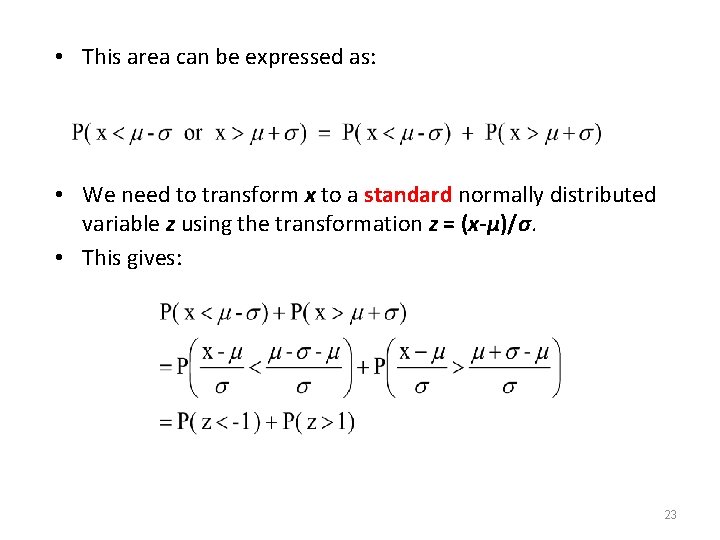
• This area can be expressed as: • We need to transform x to a standard normally distributed variable z using the transformation z = (x-μ)/σ. • This gives: 23

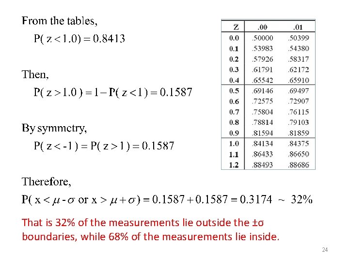
That is 32% of the measurements lie outside the ±σ boundaries, while 68% of the measurements lie inside. 24

Standard Gaussian distribution: a general rule 25

Example 4 An integrated circuit chip contains 105 transistors. The transistors have a mean current gain of 20 and a standard deviation of 2. Assuming that the current gain is normally distributed, calculate the following: (a) the number of transistors with a current gain between 19. 8 and 20. 2 (b) the number of transistors with a current gain greater than 17. 26

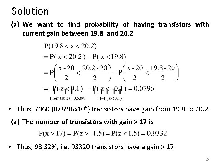
Solution (a) We want to find probability of having transistors with current gain between 19. 8 and 20. 2 • Thus, 7960 (0. 0796 x 105) transistors have gain from 19. 8 to 20. 2. (a) The number of transistors with gain > 17 is • Thus, 93. 32%, i. e. 93320 transistors have a gain > 17. 27

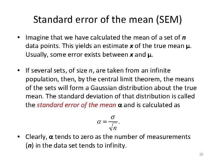
Standard error of the mean (SEM) • Imagine that we have calculated the mean of a set of n data points. This yields an estimate x of the true mean μ. Usually, some error exists between x and μ. • If several sets, of size n, are taken from an infinite population, then, by the central limit theorem, the means of the sets will form a Gaussian distribution about the true mean. The standard deviation of that distribution is called the standard error of the mean α and is calculated as • Clearly, α tends to zero as the number of measurements (n) in the data set tends to infinity. 28

Standard error of the mean (SEM) • Standard error of the mean can be used to attach a level of uncertainty to the estimated mean calculated using a finite set of measurements. • We know that a range of ± two standard deviation (i. e. , ± 2α) encompasses 95. 4% of the deviations of sample means around the true value. • Thus we can say that the true mean lies in the interval x± 2α with probability 95. 4% 29

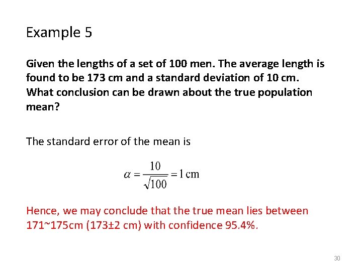
Example 5 Given the lengths of a set of 100 men. The average length is found to be 173 cm and a standard deviation of 10 cm. What conclusion can be drawn about the true population mean? The standard error of the mean is Hence, we may conclude that the true mean lies between 171~175 cm (173± 2 cm) with confidence 95. 4%. 30