8 Dynamic Programming Fibonacci sequence e g 0

§ 8 Dynamic Programming Fibonacci sequence e. g. 0 , 1 , 2 , 3 , 5 , 8 , 13 , 21 , ……. Fi = i if i 1 Fi = Fi-1 + Fi-2 if i 2 Solved by a recursive program: Much replicated computation is done. It should be solved by a simple loop. 1

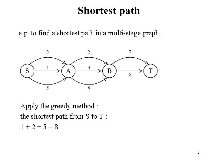
Shortest path e. g. to find a shortest path in a multi-stage graph. Apply the greedy method : the shortest path from S to T : 1+2+5=8 2

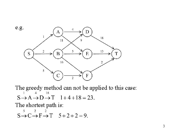
e. g. The greedy method can not be applied to this case: The shortest path is: 3

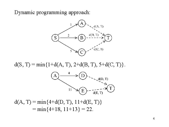
Dynamic programming approach: d(S, T) = min{1+d(A, T), 2+d(B, T), 5+d(C, T)}. d(A, T) = min{4+d(D, T), 11+d(E, T)} = min{4+18, 11+13} = 22. 4

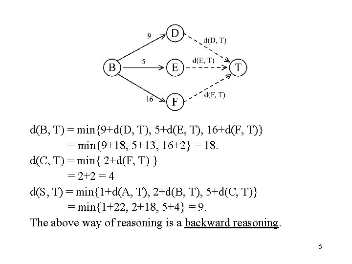
d(B, T) = min{9+d(D, T), 5+d(E, T), 16+d(F, T)} = min{9+18, 5+13, 16+2} = 18. d(C, T) = min{ 2+d(F, T) } = 2+2 = 4 d(S, T) = min{1+d(A, T), 2+d(B, T), 5+d(C, T)} = min{1+22, 2+18, 5+4} = 9. The above way of reasoning is a backward reasoning. 5

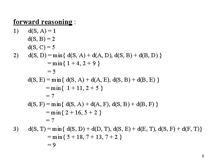
forward reasoning : 1) 2) 3) d(S, A) = 1 d(S, B) = 2 d(S, C) = 5 d(S, D) = min{ d(S, A) + d(A, D), d(S, B) + d(B, D) } = min{ 1 + 4, 2 + 9 } =5 d(S, E) = min{ d(S, A) + d(A, E), d(S, B) + d(B, E) } = min{ 1 + 11, 2 + 5 } =7 d(S, F) = min{ d(S, A) + d(A, F), d(S, B) + d(B, F) } = min{ 2 + 16, 5 + 2 } =7 d(S, T) = min{ d(S, D) + d(D, T), d(S, E) + d(E, T), d(S, F) + d(F, T)} = min{ 5 + 18, 7 + 13, 7 + 2 } =9 6

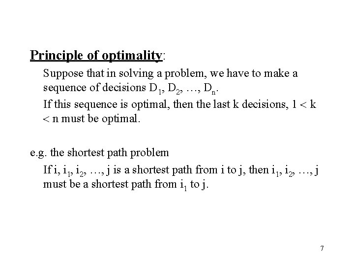
Principle of optimality: Suppose that in solving a problem, we have to make a sequence of decisions D 1, D 2, …, Dn. If this sequence is optimal, then the last k decisions, 1 k n must be optimal. e. g. the shortest path problem If i, i 1, i 2, …, j is a shortest path from i to j, then i 1, i 2, …, j must be a shortest path from i 1 to j. 7

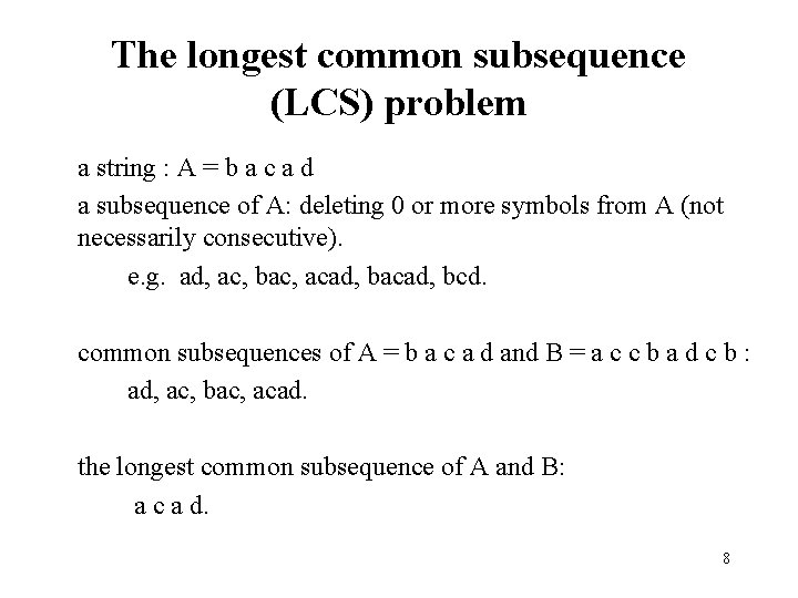
The longest common subsequence (LCS) problem a string : A = b a c a d a subsequence of A: deleting 0 or more symbols from A (not necessarily consecutive). e. g. ad, ac, bac, acad, bcd. common subsequences of A = b a c a d and B = a c c b a d c b : ad, ac, bac, acad. the longest common subsequence of A and B: a c a d. 8

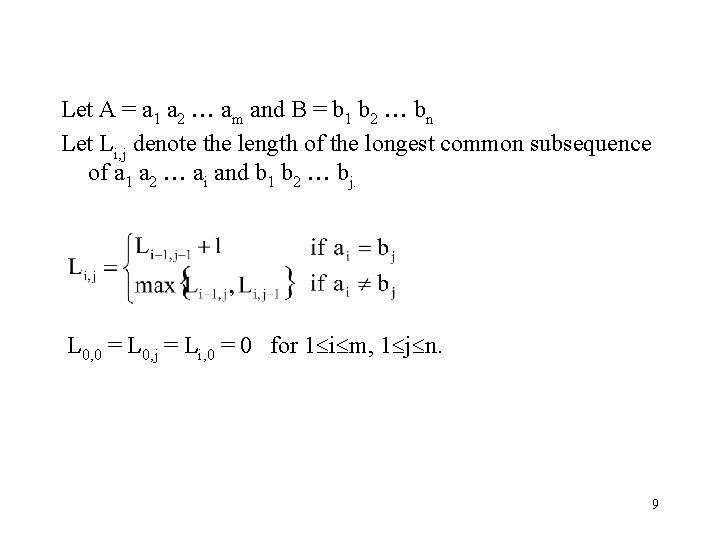
Let A = a 1 a 2 am and B = b 1 b 2 bn Let Li, j denote the length of the longest common subsequence of a 1 a 2 ai and b 1 b 2 bj. L 0, 0 = L 0, j = Li, 0 = 0 for 1 i m, 1 j n. 9

The dynamic programming approach to calculate matrix L : Time complexity : O(mn) 10

e. g. A = b a c a d, B = a c c b a d c b After all Li, j’s have been found, we can trace back to find the longest common subsequence of A and B. 11

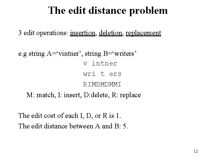
The edit distance problem 3 edit operations: insertion, deletion, replacement e. g string A=‘vintner’, string B=‘writers’ v intner wri t ers RIMDMDMMI M: match, I: insert, D: delete, R: replace The edit cost of each I, D, or R is 1. The edit distance between A and B: 5. 12

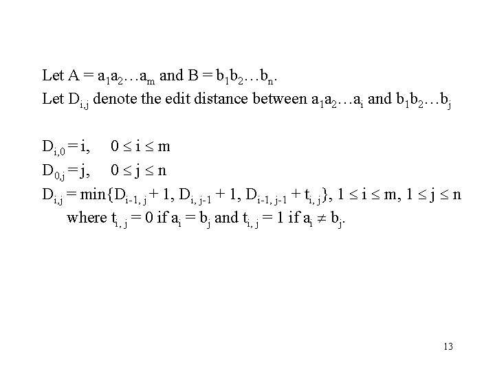
Let A = a 1 a 2…am and B = b 1 b 2…bn. Let Di, j denote the edit distance between a 1 a 2…ai and b 1 b 2…bj Di, 0 = i, 0 i m D 0, j = j, 0 j n Di, j = min{Di-1, j + 1, Di, j-1 + 1, Di-1, j-1 + ti, j}, 1 i m, 1 j n where ti, j = 0 if ai = bj and ti, j = 1 if ai bj. 13

The dynamic programming approach to calculate matrix D: time complexity: O(mn) 14

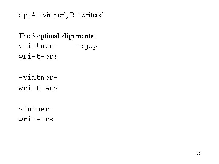
e. g. A=‘vintner’, B=‘writers’ The 3 optimal alignments : v-intner-: gap wri-t-ers -vintnerwri-t-ers vintnerwrit-ers 15

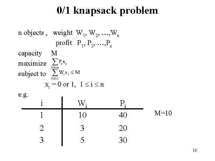
0/1 knapsack problem n objects , weight W 1, W 2, , Wn profit P 1, P 2, , Pn capacity M maximize subject to xi = 0 or 1, 1 i n e. g. i 1 Wi 10 Pi 40 2 3 3 5 20 30 M=10 16

multi-stage graph: 17

The longest path represents the optimal solution: x 1 = 0, x 2 = 1, x 3 = 1 Pixi = 20 + 30 = 50 Let fi(Q) be the value of an optimal solution to objects 1, 2, 3, …, i with capacity Q. fi(Q) = max{ fi-1(Q), fi-1(Q-Wi)+Pi } The optimal solution is fn(M). 18

Optimal binary search trees e. g. binary search trees for 3, 7, 9, 12; 19

n identifiers : a 1 <a 2 <a 3 <…< an Pi, 1 i n : the probability that ai is searched. Qi, 1 i n : the probability that x is searched where ai < x < ai+1 (a 0=- , an+1= ). internal node: successful search , Pi external node: unsuccessful search , Qi the expected cost of a binary tree: the level of the root : 1 20

e. g. identifiers : 4, 5, 8, 10, 11, 12, 14 Fig. A Binary Tree with Added External Nodes. 21

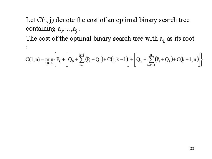
Let C(i, j) denote the cost of an optimal binary search tree containing ai, …, aj. The cost of the optimal binary search tree with ak as its root : 22

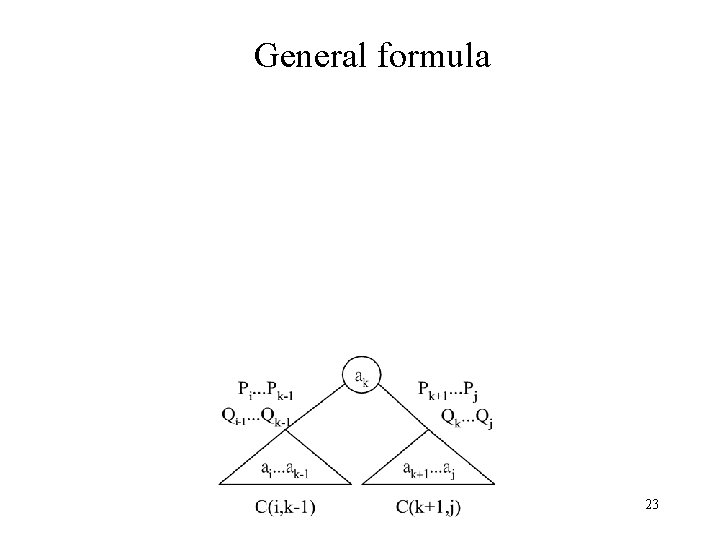
General formula 23

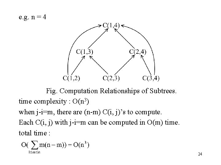
e. g. n = 4 Fig. Computation Relationships of Subtrees. time complexity : O(n 3) when j-i=m, there are (n-m) C(i, j)’s to compute. Each C(i, j) with j-i=m can be computed in O(m) time. total time : 24

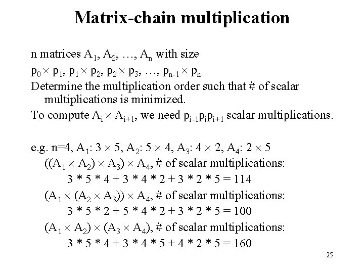
Matrix-chain multiplication n matrices A 1, A 2, …, An with size p 0 p 1, p 1 p 2, p 2 p 3, …, pn-1 pn Determine the multiplication order such that # of scalar multiplications is minimized. To compute Ai Ai+1, we need pi-1 pipi+1 scalar multiplications. e. g. n=4, A 1: 3 5, A 2: 5 4, A 3: 4 2, A 4: 2 5 ((A 1 A 2) A 3) A 4, # of scalar multiplications: 3 * 5 * 4 + 3 * 4 * 2 + 3 * 2 * 5 = 114 (A 1 (A 2 A 3)) A 4, # of scalar multiplications: 3 * 5 * 2 + 5 * 4 * 2 + 3 * 2 * 5 = 100 (A 1 A 2) (A 3 A 4), # of scalar multiplications: 3 * 5 * 4 + 3 * 4 * 5 + 4 * 2 * 5 = 160 25

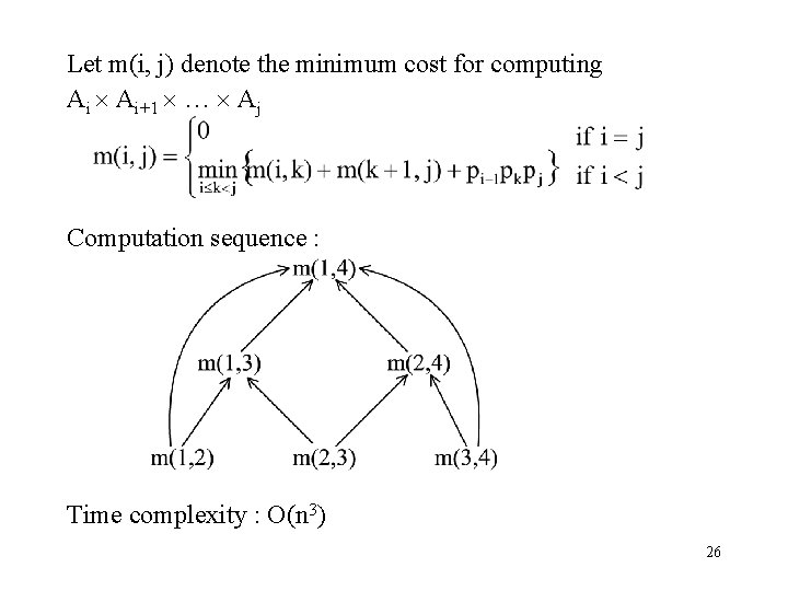
Let m(i, j) denote the minimum cost for computing Ai Ai+1 … Aj Computation sequence : Time complexity : O(n 3) 26