8 4 The Normal Distribution Understand the basic

8. 4 The Normal Distribution • Understand the basic properties of the normal curve. • Relate the area under a normal curve to z-scores. • Make conversions between raw scores and z-scores. • Use the normal distribution to solve applied problems.

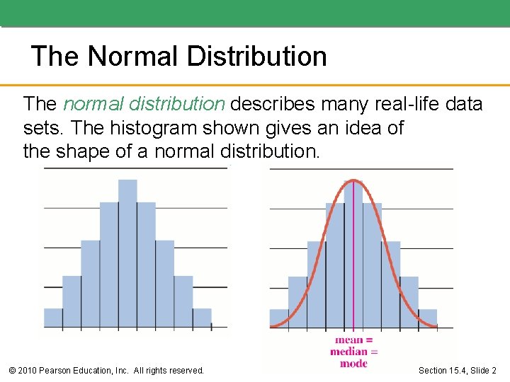
The Normal Distribution The normal distribution describes many real-life data sets. The histogram shown gives an idea of the shape of a normal distribution. © 2010 Pearson Education, Inc. All rights reserved. Section 15. 4, Slide 2

The Normal Distribution © 2010 Pearson Education, Inc. All rights reserved. Section 15. 4,

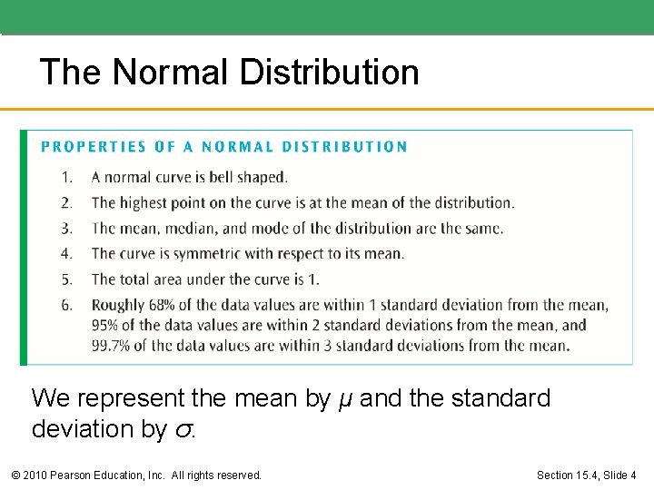
The Normal Distribution We represent the mean by μ and the standard deviation by

The Normal Distribution • Example: Suppose that the distribution of scores of 1, 000 students who take a standardized intelligence test is a normal distribution. If the distribution’s mean is 450 and its standard deviation is 25, a) how many scores do we expect to fall between 425 and 475? b) how many scores do we expect to fall above 500? (continued on next slide) © 2010 Pearson Education, Inc. All rights reserved. Section 15. 4, Slide 5

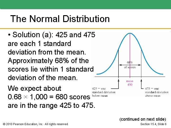
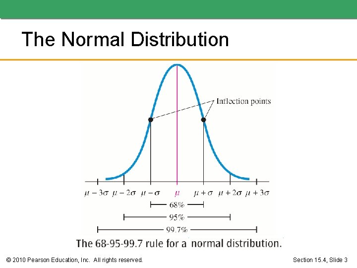
The Normal Distribution • Solution (a): 425 and 475 are each 1 standard deviation from the mean. Approximately 68% of the scores lie within 1 standard deviation of the mean. We expect about 0. 68 × 1, 000 = 680 scores are in the range 425 to 475. (continued on next slide) © 2010 Pearson Education, Inc. All rights reserved. Section 15. 4, Slide 6

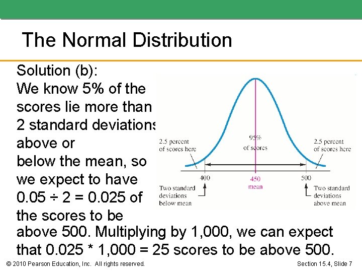
The Normal Distribution Solution (b): We know 5% of the scores lie more than 2 standard deviations above or below the mean, so we expect to have 0. 05 ÷ 2 = 0. 025 of the scores to be above 500. Multiplying by 1, 000, we can expect that 0. 025 * 1, 000 = 25 scores to be above 500. © 2010 Pearson Education, Inc. All rights reserved. Section 15. 4, Slide 7

z-Scores The standard normal distribution has a mean of 0 and a standard deviation of 1. There are tables (see next slide) that give the area under this curve between the mean and a number called a z-score. A z-score represents the number of standard deviations a data value is from the mean. For example, for a normal distribution with mean 450 and standard deviation 25, the value 500 is 2 standard deviations above the mean; that is, the value 500 corresponds to a z-score of 2. © 2010 Pearson Education, Inc. All rights reserved. Section 15. 4, Slide 8

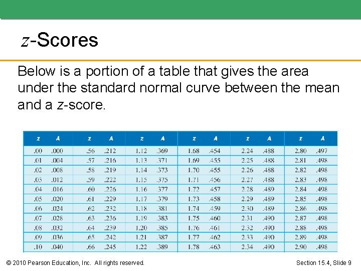
z-Scores Below is a portion of a table that gives the area under the

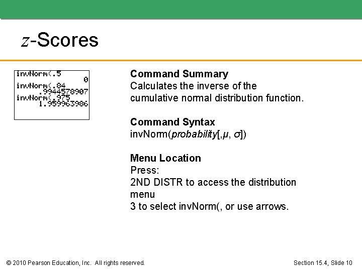
z-Scores Command Summary Calculates the inverse of the cumulative normal distribution function. Command Syntax inv. Norm(probability[, μ, σ]) Menu Location Press: 2 ND DISTR to access the distribution menu 3 to select inv. Norm(, or use arrows. © 2010 Pearson Education, Inc. All rights reserved. Section 15. 4, Slide 10

z-Scores • Example: Use a table to find the percentage of the data (area under the curve) that lie in the following regions for a standard normal distribution: a) between z = 0 and z = 1. 3 b) between z = 1. 5 and z = 2. 1 c) between z = 0 and z = – 1. 83 (continued on next slide) © 2010 Pearson Education, Inc. All rights reserved. Section 15. 4, Slide 11

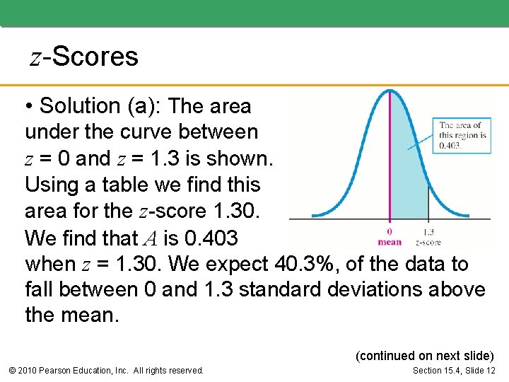
z-Scores • Solution (a): The area under the curve between z = 0 and z = 1. 3 is shown. Using a table we find this area for the z-score 1. 30. We find that A is 0. 403 when z = 1. 30. We expect 40. 3%, of the data to fall between 0 and 1. 3 standard deviations above the mean. (continued on next slide) © 2010 Pearson Education, Inc. All rights reserved. Section 15. 4, Slide 12

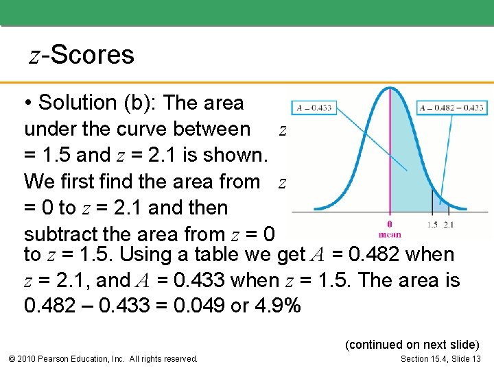
z-Scores • Solution (b): The area under the curve between z = 1. 5 and z = 2. 1 is shown. We first find the area from z = 0 to z = 2. 1 and then subtract the area from z = 0 to z = 1. 5. Using a table we get A = 0. 482 when z = 2. 1, and A = 0. 433 when z = 1. 5. The area is 0. 482 – 0. 433 = 0. 049 or 4. 9% (continued on next slide) © 2010 Pearson Education, Inc. All rights reserved. Section 15. 4, Slide 13

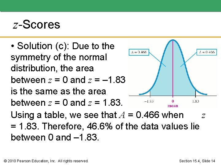
z-Scores • Solution (c): Due to the symmetry of the normal distribution, the area between z = 0 and z = – 1. 83 is the same as the area between z = 0 and z = 1. 83. Using a table, we see that A = 0. 466 when z = 1. 83. Therefore, 46. 6% of the data values lie between 0 and – 1. 83. © 2010 Pearson Education, Inc. All rights reserved. Section 15. 4, Slide 14

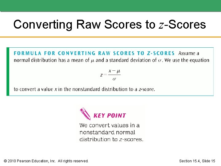
Converting Raw Scores to z-Scores © 2010 Pearson Education, Inc. All rights reserved. Section

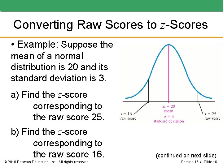
Converting Raw Scores to z-Scores • Example: Suppose the mean of a normal distribution is 20 and its standard deviation is 3. a) Find the z-score corresponding to the raw score 25. b) Find the z-score corresponding to the raw score 16. © 2010 Pearson Education, Inc. All rights reserved. (continued on next slide) Section 15. 4, Slide 16

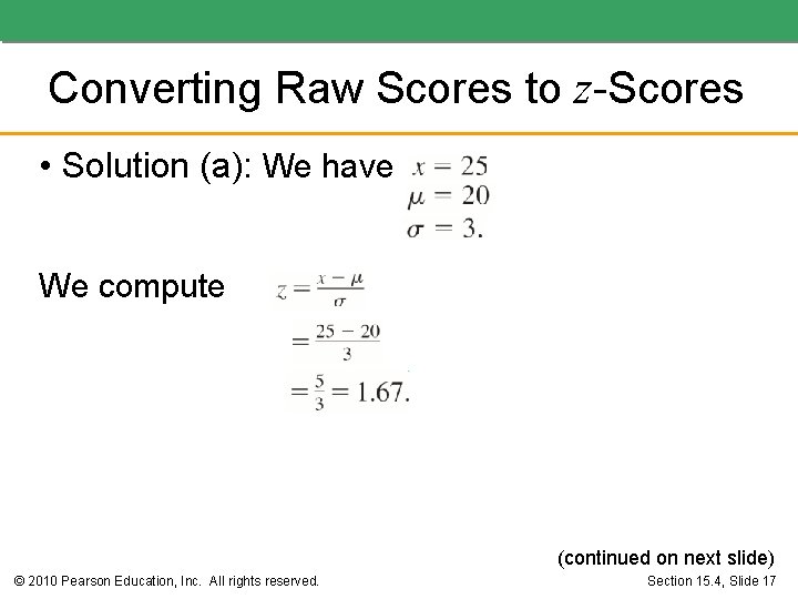
Converting Raw Scores to z-Scores • Solution (a): We have We compute (continued on

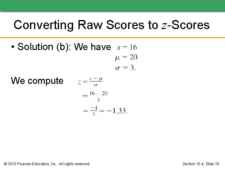
Converting Raw Scores to z-Scores • Solution (b): We have We compute © 2010

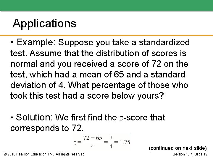
Applications • Example: Suppose you take a standardized test. Assume that the distribution of scores is normal and you received a score of 72 on the test, which had a mean of 65 and a standard deviation of 4. What percentage of those who took this test had a score below yours? • Solution: We first find the z-score that corresponds to 72. (continued on next slide) © 2010 Pearson Education, Inc. All rights reserved. Section 15. 4, Slide 19

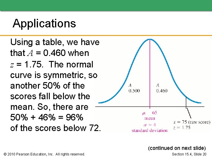
Applications Using a table, we have that A = 0. 460 when z = 1. 75. The normal curve is symmetric, so another 50% of the scores fall below the mean. So, there are 50% + 46% = 96% of the scores below 72. (continued on next slide) © 2010 Pearson Education, Inc. All rights reserved. Section 15. 4, Slide 20

Applications • Example: Consider the following information: 1911: Ty Cobb hit. 420. Mean average was. 266 with standard deviation. 0371. 1941: Ted Williams hit. 406. Mean average was. 267 with standard deviation. 0326. 1980: George Brett hit. 390. Mean average was. 261 with standard deviation. 0317. Assuming normal distributions, use z-scores to determine which of the three batters was ranked (continued on next slide) the highest in relationship to his contemporaries. © 2010 Pearson Education, Inc. All rights reserved. Section 15. 4, Slide 21

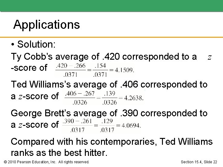
Applications • Solution: Ty Cobb’s average of. 420 corresponded to a -score of z Ted Williams’s average of. 406 corresponded to a z-score of George Brett’s average of. 390 corresponded to a z-score of Compared with his contemporaries, Ted Williams ranks as the best hitter. © 2010 Pearson Education, Inc. All rights reserved. Section 15. 4, Slide 22

Applications • Example: A manufacturer plans to offer a warranty on an electronic device. Quality control engineers found that the device has a mean time to failure of 3, 000 hours with a standard deviation of 500 hours. Assume that the typical purchaser will use the device for 4 hours per day. If the manufacturer does not want more than 5% to be returned as defective within the warranty period, how long should the warranty period be to guarantee this? (continued on next slide) © 2010 Pearson Education, Inc. All rights reserved. Section 15. 4, Slide 23

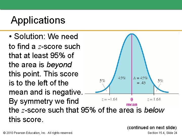
Applications • Solution: We need to find a z-score such that at least 95% of the area is beyond this point. This score is to the left of the mean and is negative. By symmetry we find the z-score such that 95% of the area is below this score. (continued on next slide) © 2010 Pearson Education, Inc. All rights reserved. Section 15. 4, Slide 24

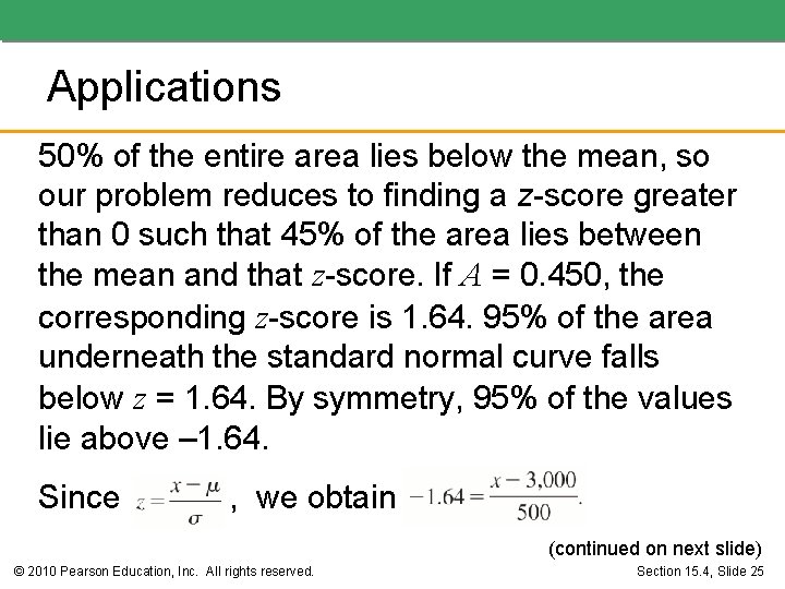
Applications 50% of the entire area lies below the mean, so our problem reduces to finding a z-score greater than 0 such that 45% of the area lies between the mean and that z-score. If A = 0. 450, the corresponding z-score is 1. 64. 95% of the area underneath the standard normal curve falls below z = 1. 64. By symmetry, 95% of the values lie above – 1. 64. Since , we obtain (continued on next slide) © 2010 Pearson Education, Inc. All rights reserved. Section 15. 4, Slide 25

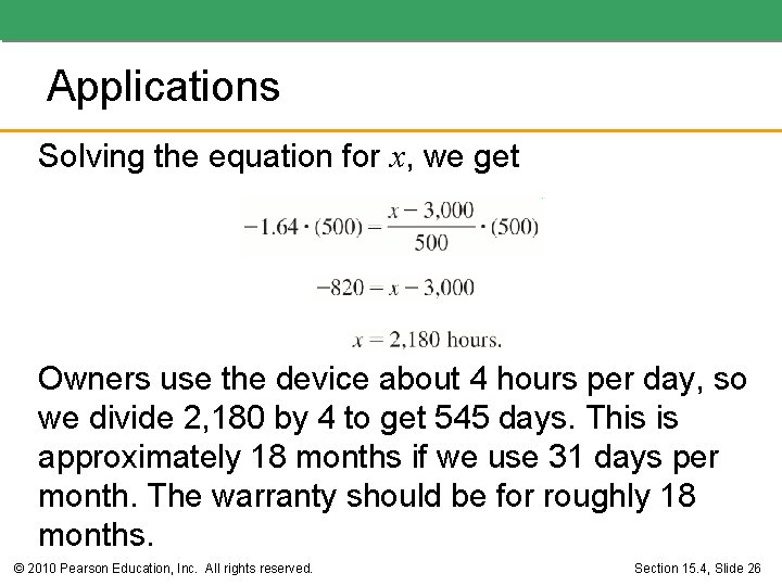
Applications Solving the equation for x, we get Owners use the device about 4 hours per day, so we divide 2, 180 by 4 to get 545 days. This is approximately 18 months if we use 31 days per month. The warranty should be for roughly 18 months. © 2010 Pearson Education, Inc. All rights reserved. Section 15. 4, Slide 26