7 Metropolis Algorithm Markov Chain and Monte Carlo

7. Metropolis Algorithm

Markov Chain and Monte Carlo • Markov chain theory describes a particularly simple type of stochastic processes. Given a transition matrix, W, the invariant distribution P can be determined. • Monte Carlo is a computer implementation of a Markov chain. In Monte Carlo, P is given, we need to find W such that P = P W.

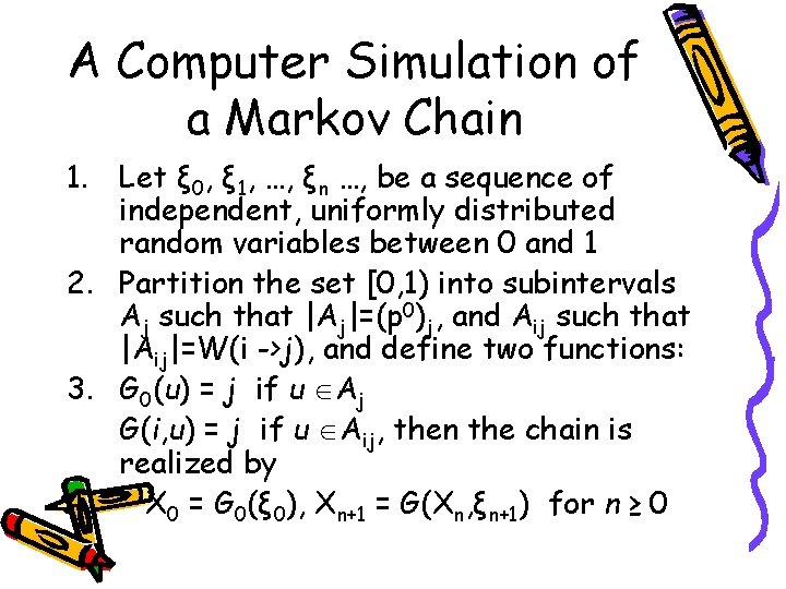
A Computer Simulation of a Markov Chain 1. Let ξ 0, ξ 1, …, ξn …, be a sequence of independent, uniformly distributed random variables between 0 and 1 2. Partition the set [0, 1) into subintervals Aj such that |Aj|=(p 0)j, and Aij such that |Aij|=W(i ->j), and define two functions: 3. G 0(u) = j if u Aj G(i, u) = j if u Aij, then the chain is realized by 4. X 0 = G 0(ξ 0), Xn+1 = G(Xn, ξn+1) for n ≥ 0

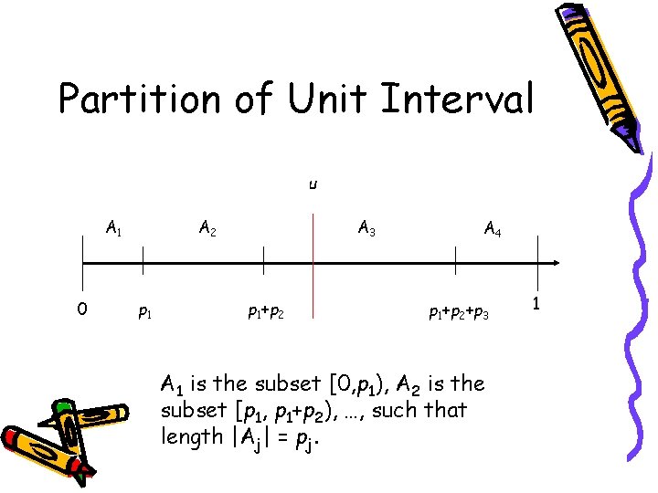
Partition of Unit Interval u A 1 0 A 2 p 1 A 3 p 1+p 2 A 4 p 1+p 2+p 3 A 1 is the subset [0, p 1), A 2 is the subset [p 1, p 1+p 2), …, such that length |Aj| = pj. 1

Markov Chain Monte Carlo • Generate a sequence of states X 0, X 1, …, Xn, such that the limiting distribution is given by P(X) • Move X by the transition probability W(X -> X’) • Starting from arbitrary P 0(X), we have Pn+1(X) = ∑X’ Pn(X’) W(X’ -> X) • Pn(X) approaches P(X) as n go to ∞

Necessary and sufficient conditions for convergence • Ergodicity [Wn](X - > X’) > 0 For all n > nmax, all X and X’ • Detailed Balance P(X) W(X -> X’) = P(X’) W(X’ -> X)

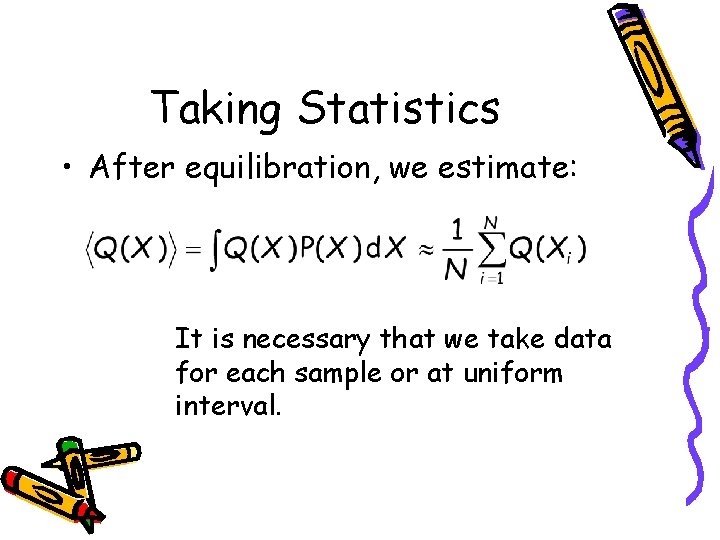
Taking Statistics • After equilibration, we estimate: It is necessary that we take data for each sample or at uniform interval.

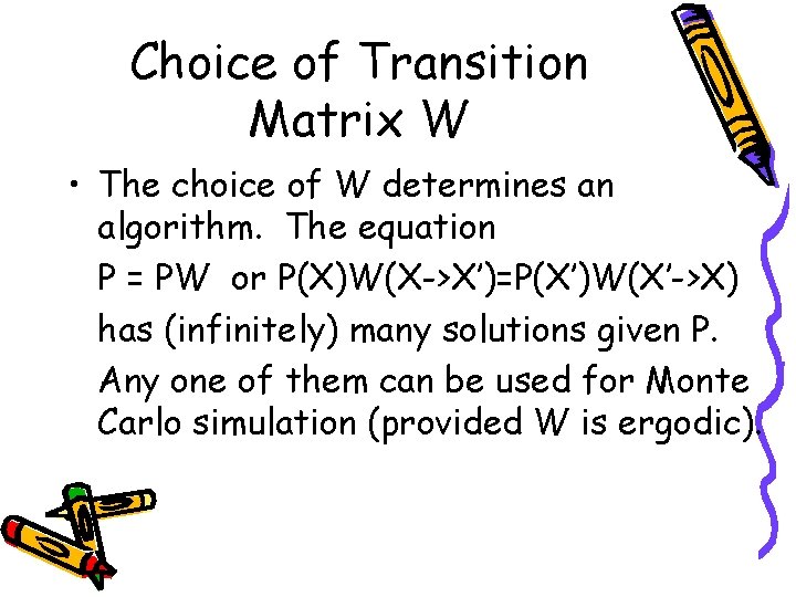
Choice of Transition Matrix W • The choice of W determines an algorithm. The equation P = PW or P(X)W(X->X’)=P(X’)W(X’->X) has (infinitely) many solutions given P. Any one of them can be used for Monte Carlo simulation (provided W is ergodic).

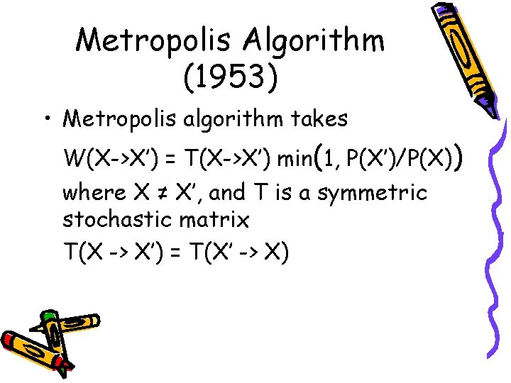
Metropolis Algorithm (1953) • Metropolis algorithm takes W(X->X’) = T(X->X’) min(1, P(X’)/P(X)) where X ≠ X’, and T is a symmetric stochastic matrix T(X -> X’) = T(X’ -> X)

The Paper (42500 citations up to 2020) THE JOURNAL OF CHEMICAL PHYSICS VOLUME 21, NUMBER 6 JUNE, 1953 Equation of State Calculations by Fast Computing Machines NICHOLAS METROPOLIS, ARIANNA W. ROSENBLUTH, MARSHALL N. ROSENBLUTH, AND AUGUSTA H. TELLER, Los Alamos Scientific Laboratory, Los Alamos, New Mexico AND EDWARD TELLER, * Department of Physics, University of Chicago, Illinois (Received March 6, 1953) A general method, suitable for fast computing machines, for investigating such properties as equations of state for substances consisting of interacting individual molecules is described. The method consists of a modified Monte Carlo integration over configuration space. Results for the two-dimensional rigid-sphere system have been obtained on the Los Alamos MANIAC and are presented here. These results are compared to the free volume equation of state and to a four-term virial coefficient expansion. 1087

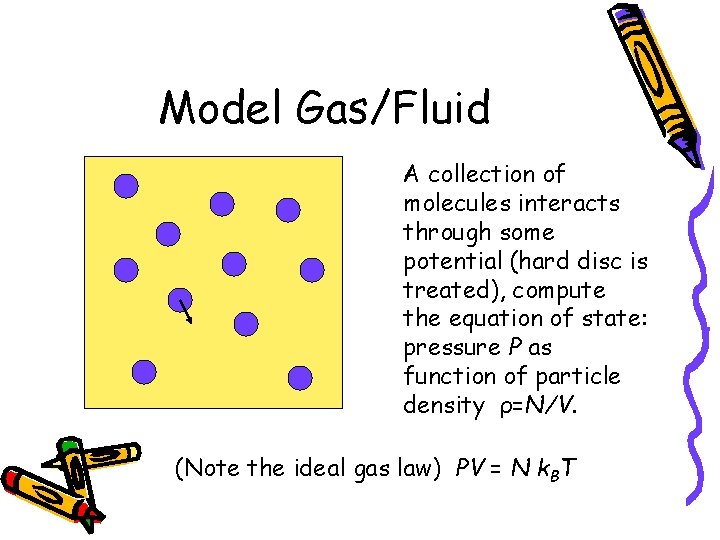
Model Gas/Fluid A collection of molecules interacts through some potential (hard disc is treated), compute the equation of state: pressure P as function of particle density ρ=N/V. (Note the ideal gas law) PV = N k. BT

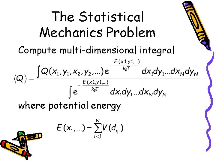
The Statistical Mechanics Problem Compute multi-dimensional integral where potential energy

Importance Sampling “…, instead of choosing configurations randomly, …, we choose configuration with a probability exp(-E/k. BT) and weight them evenly. ” - from M(RT)2 paper

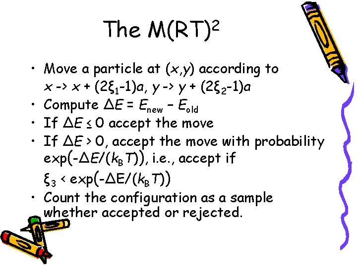
The M(RT)2 • Move a particle at (x, y) according to x -> x + (2ξ 1 -1)a, y -> y + (2ξ 2 -1)a • Compute ΔE = Enew – Eold • If ΔE ≤ 0 accept the move • If ΔE > 0, accept the move with probability exp(-ΔE/(k. BT)), i. e. , accept if ξ 3 < exp(-ΔE/(k. BT)) • Count the configuration as a sample whether accepted or rejected.

A Priori Probability T • What is T(X->X’) in the Metropolis algorithm? • And why it is symmetric?

The Calculation • Number of particles N = 224 • Monte Carlo sweep ≈ 60 • Each sweep took 3 minutes on MANIAC • Each data point took 5 hours

MANIAC the Computer and the Man Seated is Nick Metropolis, the background is the MANIAC vacuum tube computer

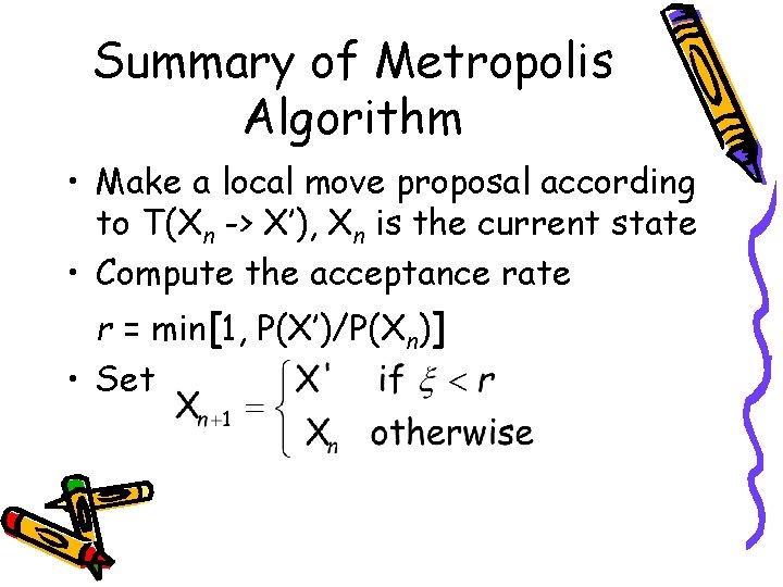
Summary of Metropolis Algorithm • Make a local move proposal according to T(Xn -> X’), Xn is the current state • Compute the acceptance rate r = min[1, P(X’)/P(Xn)] • Set

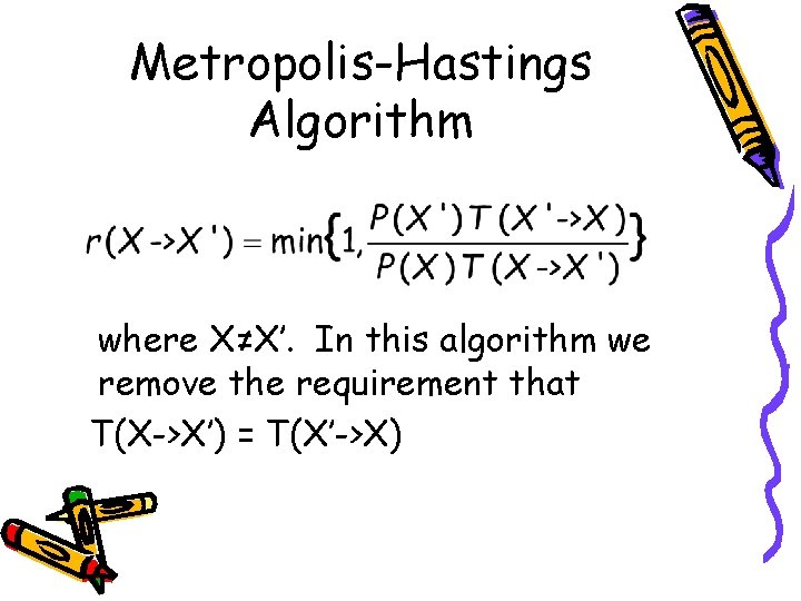
Metropolis-Hastings Algorithm where X≠X’. In this algorithm we remove the requirement that T(X->X’) = T(X’->X)

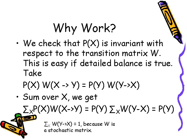
Why Work? • We check that P(X) is invariant with respect to the transition matrix W. This is easy if detailed balance is true. Take P(X) W(X -> Y) = P(Y) W(Y->X) • Sum over X, we get ∑XP(X)W(X->Y) = P(Y) ∑XW(Y-X) = P(Y) ∑X W(Y->X) = 1, because W is a stochastic matrix.

Detailed Balance Satisfied • For X≠Y, we have W(X->Y) = T(X->Y) min[1, P(Y)T(Y->X)/(P(X)T(X->Y)) ] • So if P(X)T(X->Y) > P(Y)T(Y->X), we get P(X)W(X->Y) = P(Y) T(Y->X), and P(Y)W(Y->X) = P(Y) T(Y->X) • Same is true when the inequality is reversed. Detailed balance means P(X)W(X->Y) = P(Y) W(Y->X)

Ergodicity • The unspecified part of Metropolis algorithm is T(X->X’), the choice of which determines if the Markov chain is ergodic. • Choice of T(X->X’) is problem specific. We can adjust T(X->X’) such that acceptance rate r ≈ 0. 23

Gibbs Sampler or Heat. Bath Algorithm • If X is a collection of components, X=(x 1, x 2, …, xi, …, x. N), and if we can compute P(xi|x 1, …, xi-1, xi+1, . . , x. N), we generate the new configuration by sampling xi according to the above conditional probability.