7 Eigenvalue Problems 7 1 Introduction Jacobi method

7. Eigenvalue Problems
")
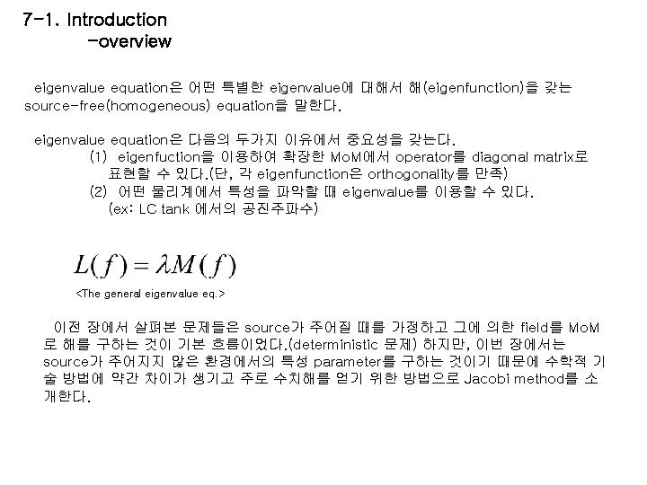
7 -1. Introduction -Jacobi method (Appendix. C)

7 -2. Method of Moments -overview 실제로 eigenvalue eq. 을 풀기 위한 Mo. M의 적용은 이전의 deterministic eq. 에 대한 Mo. M의 적용과 방식은 거의 유사하다. (functional equation form) (matrix equation form)
를")
7 -2. Method of Moments -Example 이 예제는 간단한 경우(eigenfunction, eigenvalue가 쉽게 구해지는 경우)를 예로 든 것이다. 즉, exact solution과 Mo. M을 이용하여 구한 solution을 비교해 본다. (i) Exact solution ; (ii) Mo. M solution ; 두 확장함수(eigenfunction)을 비교해 보면 첫번째의 경우, orthogonal하지만 두번째의 경우에는 orthogonal 하지 않다.
")
7 -2. Method of Moments -Example (Cont. )
, c(x)는")
7 -3. Nonuniform Transmission Line -overview loss-free transmission line이고 timeharmonic case임을 밝힌다. l(x), c(x)는 각각 단위길이당 series ind. , shunt cap. 이다. 그러면 이제 transmission line eq. 을 구해보 자. 주의할 점은 c와 l은 미분가능함을 전제로 유도 할 것이다.
 여기서 단위길이당 L과 C는 distribute, 미분가능으로")
7 -3. Nonuniform Transmission Line -overview (Cont. ) 여기서 단위길이당 L과 C는 distribute, 미분가능으로 가정되어 있기 때문에 최종적으로 만들어진 eigenvalue equation 의 operator는 non-self-adjoint operator이다. 즉, 일반적인 물리 법칙에서 위배되는 해를 만들어 낼 수 있다. 그래서 다음 절에서는 이를 self-adjoint operator 로 만드는 과정과 예제를 다룬다. 참고로 wave equation에서는 “k”가 operator의 domain과 independent하므로 self-adjoint operator가 된다.

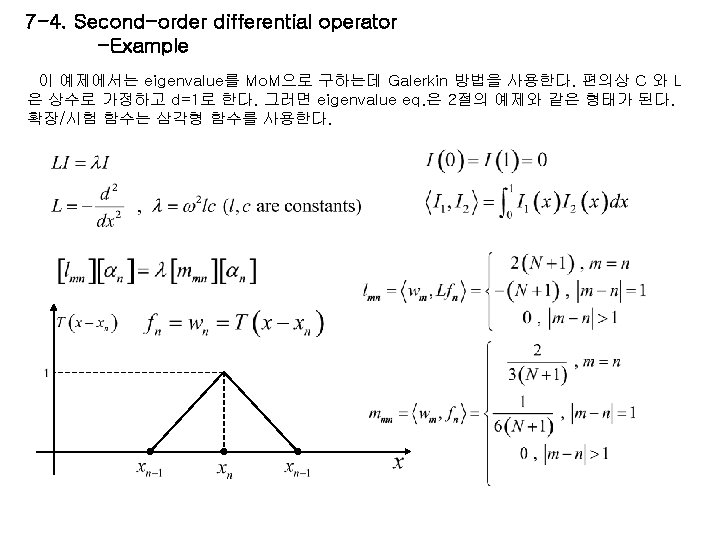
7 -4. Second-order differential operator -overview 계속되는 예는 3절의 transmission line이다. Transmission line eq. 이 eigenvalue eq. 이고 이 방정식의 해는 결국 transmission line의 공진 주파수로서 real 값을 가질 것이다. 그러므 로 eigenvalue eq. 의 operator는 Hermitian operator여야 한다. 그러나 앞서 살펴본 결과, operator는 non-self-adjoint 이다. 이를 적절히 바꿔서 boundary condition을 만족하는 self-adjoint operator로 만든다. 참고로 Hermitian operator는 (1) self-adjoint operator이 고, (2) operator의 boundary condition을 각 함수가 만족할 경우의 operator를 일컫는다. 먼저 Hermitian operator를 갖는 Sturm-Liouville eq. 과 비교하여 normalizing 함수를 구하 는 방식으로 self-adjoint operator로 만든다.
")
7 -4. Second-order differential operator -overview (Cont. )

7 -5. First-order differential operator -overview A second-order differential equation can be expressed as a pair of first-order differential equations. (ex : transmission line problem) 결국 이 절의 목표는 어떤 정확한 eigenfunction을 구하는 데에 2차 미분 방정식의 수치 해 보다 1차 미분 방정식의 수치해가 더욱 빨리 수렴하기 때문에 2차 미분 방정식을 1차 미 분 방정식의 쌍으로 표현하여 수치해를 구하는 것이다.

7 -5. First-order differential operator -Example A & B
")
7 -5. First-order differential operator -Example A & B (Cont. )

7 -6. Extended operator -Example
- Slides: 16