7 Differences between more than two samples Oneway

7. Differences between more than two samples One-way analysis of variance Kruskal-Wallis oneway analysis Two-way analysis of variance Normally distributed data Alternative models of analysis of variance Ranks for data
 of two")
독립표본 T-test Independent Sample T-test t test Compared the means (or medians) of two samples 독립표본 T-test는 데이터가 서로 다른 두 모 집단으로부터 추출된 경우에 사용하는 분석 방법으로, 분석결과의 해석은 T 값, p-value, 95% 신 뢰 구 간 등 을 활 용 할 수 있 음. Compare two different data set Mann-Whitney U test But many experiments or surveys Comparison of three or more samples

Example Loft insulation Double-glazing insulation Minimal insulation Electricity consumption in winter Effect of insulation Household energy bill “Loft insulation” with “Double-glazing insulation” “Loft insulation” with “Minimal insulation” Perform three “t” tests “Double-glazing insulation” with “Minimal insulation” Very long-winded computation & timeconsuming Seven samples 21 separate tests

More serious objection Conducting multiple t tests Compute several tests Increase the chances of getting significant result by chance alone For multiple t tests with probability value 0. 05 (the value reject null hypothesis) Only 5% probability of null hypothesis of result occurred by chance Its mean 5% of occasions the null hypothesis is rejected Type I error (see Chapter 3) If we do 20 tests At least one significant result even if there were no real differences between means
 Committing")
To solve the above problem Simultaneously compare three or more means (or medians) Committing a type I error Simultaneously compare Normally distributed data Use parametric analysis of variance (ANOVA) One-way analysis of variance. Two-way analysis of variance. Depends on experiment Three-way analysis of variance
 One-way analysis of variance Two-way analysis of variance")
Use parametric analysis of variance (ANOVA) One-way analysis of variance Two-way analysis of variance One independent variable One dependent variable Electricity consumption Energy (electricity) bill In one-way ANOVA Seoul (more cold) Electricity consumption Energy (electricity) bill Data from Busan (less cold) Climate difference in two areas Not true results
 Electricity consumption Energy (electricity) bill Data from")
In one-way ANOVA Seoul (more cold) Electricity consumption Energy (electricity) bill Data from Busan (less cold) Climate difference in two areas Not true results Insulation type In this case Two independent variables City Two-way analysis of variance

Experiment 1 Example not in book 10 worms each Experiment Control Cadmium Soil 1 Replication One independe nt variable (Cd conc. ) One dependent variable (EW growth) R 2 R 3 One-way Anova 0 Cd 0. 1 Cd 10 Concentration - ppm

Experiment 1 Example not in book 10 worms each Experiment Control Cadmium Soil 2 R 1 Replication One independe nt variable (Cd conc. ) One dependent variable (EW growth) R 2 R 3 One-way Anova 0 Cd 0. 1 Cd 10 Concentration - ppm

Example not in book Soil 1 0 Cd 0. 1 Cd 1 Two-way Anova Cd 10 0 Soil 2 Cd 0. 1 Cd 10 Two independent variables One dependent variables Cd concentration & Soil type Earthworm growth

If data measured in ordinal scale Kruskal-Wallis one-way analysis of variance using ranks One-way analyses of variance (parametric and then nonparametric tests) Two-way analyses (again both parametric and nonparametric tests). Parametric analysis to test group means 평균 Nonparametric analysis to test group medians 중앙값

Parametric one-way analysis of variance Test group means 평균 In one-way ANOVA Electricity consumption Energy (electricity) bill Many factors influence Type of heating system How many hours heated How many rooms heated One-way ANOVA effectively calculates the test statistic (F) ratio of explained to unexplained variation
 Homoscedasticity assumption : variance around the regression line")
Testing for equality of variances (Homoscedasticity) Homoscedasticity assumption : variance around the regression line is the same for all values of the predictor variable (X). The plot shows a violation 위반 of this assumption. For the lower values on the X-axis, the points are all very near the regression line. For the higher values on the X-axis, there is much more variability around the regression line. Not in book

First Variances obtained for each sample Then, largest variance compared with smallest If no significantly different between smallest & largest values the other values not significantly differed Largest variance ----------- = Fmax Smallest variance Fmax value compared to a table of critical values of F
 IN HOUSES")
WORKED EXAMPLE 7. 1 A ANOVA FOR ENERGY BILLS (£ PER ANNUM) IN HOUSES WITH DIFFERENT TYPES OF INSULATION: CALCULATING THE FMAX TEST
2 149 -164. 37 =")
Loft Insulation Value - Average 149 Average (Value – Average)2 149 -164. 37 = -15. 3 234. 09 198 33. 7 1135. 69 179 14. 7 216. 09 158 -6. 3 39. 69 134 -30. 3 918. 09 155 -9. 3 86. 49 181 16. 7 278. 89 161 -3. 3 10. 89 1315 164. 37 2919. 92 ------df (8 -1) = 7 417. 13

417. 13
2 134 -171. 5 = -37. 5")
Value - Average 134 Average (Value – Average)2 134 -171. 5 = -37. 5 1406. 25 181 9. 5 90. 25 198 26. 5 702. 25 187 15. 5 240. 25 151 -20. 5 420. 25 174 2. 5 6. 25 178 6. 5 42. 25 169 -2. 5 6. 25 1372 171. 5 2914 ------df (8 -1) = 7 416. 28

417. 13 416. 3

Largest variance Fmax = ----------- Smallest variance 417. 13 Fmax = ------ = 1. 109 376. 00 417. 13 416. 3 376
 < table value P=0. 05 (i. e.")
If the calculated value (1. 109 ) < table value P=0. 05 (i. e. P≥ 0. 05) Accept null hypothesis no significant difference If the calculated value (1. 109 ) > table value Significantly different (P<0. 05) Number of sample comparing = 3 Degrees of freedom (8 -1) = 7

Table 7. 1 Selected values of Fmax for testing equality of variances. Reject the null hypothesis if the calculated value of Fmax is greater than the table value. Values are given for P=0. 05. Shaded lines indicate the critical values for the example referred to in the text. A more comprehensive table of F values is given in Table D. 9 (Appendix D) Page 202 If the calculated value (1. 109 ) < table value 6. 94 Accept null hypothesis no significant difference Safe to proceed with the ANOVA

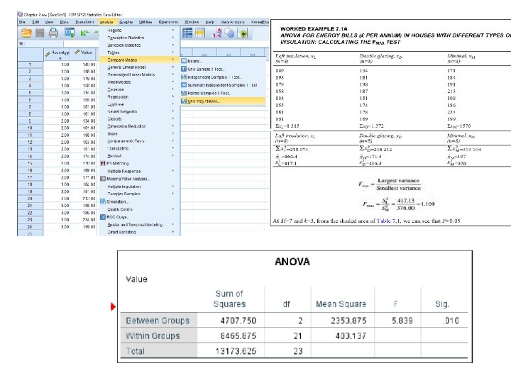
Calculating the F statistic for ANOVA First finding total variation in the data Explained variation (Between variation, or SSbetween) Sums of squares Unexplained variation (Within variation, or SSwithin) SStotal = SSbetween + SSwithin The formulae for calculating the sums of squares are shown in Box 7. 1, and the calculations for the energy example are shown in Worked Example 7. 1 b.

BOX 7. 1 FORMULAE FOR THE SUMS OF SQUARES FOR ANOVA The sum of squares of all the data points is: Σx. T - sum of all values in all samples n. T - total number of values in all samples Within variation is the sum of variation in the individual samples

Between sample sum of squares Total sum of squares Sum of all values in sample 1 Sum of all values in sample 2 n 1 number of values n 2 number of values
 IN HOUSES")
WORKED EXAMPLE 7. 1 B ANOVA FOR ENERGY BILLS (£ PER ANNUM) IN HOUSES WITH DIFFERENT TYPES OF INSULATION: CALCULATING THE SUMS OF SQUARES USING THE DATA FROM WORKED EXAMPLE 7. 1 A Lot insulation Sum 149 198 179 158 134 155 181 161 1315 Double glazing Sum 2 22201 39204 32041 24964 17956 24025 32761 25921 134 181 198 187 151 174 178 169 2 17956 32761 39204 34969 22801 30276 31684 28561 219073 1372 238212 Minimal Sum 171 184 191 213 198 186 234 199 2 29241 33856 36481 45369 39204 34596 54756 39601 1576 313104

Total Average Previous slide Total sum of squares Calculated for Fmax

Sum of squares for each sample

Calculate SSwithin & SSbetween Check calculations, confirm the total 13173 calculated in previous slide

Output from statistical software Degrees of freedom Total degrees of freedom = (Total number of data points -1) Between degrees of freedom = (Number of samples - 1) Within degrees of freedom = Total df - between df
 Statistic, F, MSbetween (explained) ---------------Mswithin (unexplained) Test statistic")
Sums of squares Mean square (MS) Statistic, F, MSbetween (explained) ---------------Mswithin (unexplained) Test statistic is then compared to table values of F Using two values of degrees of freedom (between & within) Probability 가능성, 확률 Based on this value we can decide whether it is significant or not
 is not significantly greater than the unexplained variation")
Null hypothesis Explained variation (between variation) is not significantly greater than the unexplained variation (within variation) Alternative hypothesis Explained variation is > unexplained variation
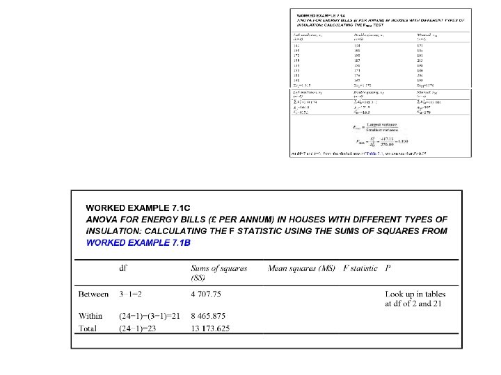

Table 7. 3 Selected values of the F distribution for ANOVA. Reject null hypothesis if the calculated values of F are greater than the table values. The upper (bold) figures are for P=0. 05, while the lower figures are for P— 0. 01. Shading indicates the critical values for the example referred to In the text. A more comprehensive table of F values is given in Table D. 7 (Appendix D) Page 200 Calculated F value (5. 839) exceeds the table value for both P =0. 05 (F=3. 47) and P=0. 01 (F=5. 78) Reject the null hypothesis Accept the alternative hypothesis
 has a highly significant effect")
Insulation category (whether loft insulation, double-glazing or minimal insulation) has a highly significant effect on household energy bills (F 2, 21=5. 839, P<0. 01).

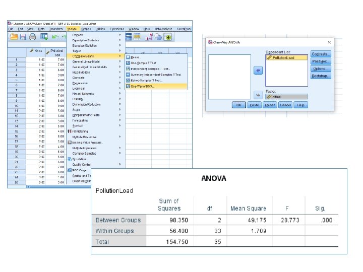
Example Not in Book Pollution level in 3 cities Sample Busan Daegu Seoul 1 7 5 1 2 7 6 3 3 6 3 4 4 9 5 3 5 8 4 1 6 7 6 1 7 6 5 2 8 7 4 6 9 8 5 5 10 9 5 4 11 6 3 12 7 4 13 6 5 13 13 n 10 ntotal Mean ( x) Total k (number of cities) 10+13+13= 36 7. 4 5. 15 3. 23 All values / 36 = 5. 08 (If sample size is equal 7. 4+5. 15+3. 23/3, not fit here) 3 Null hypothesis (HO) Busan = Daegu = Seoul Alternative hypothesis (H 1) Busan ≠ Daegu ≠ Seoul P=0. 05
2 (x 2 -x )2 (x 3")
Sample Busan Daegu Seoul (x 1 -x )2 (x 2 -x )2 (x 3 -x )2 1 7 5 1 (7 -7. 4)2=0. 16 2 7 6 3 0. 16 0. 72 0. 05 3 6 3 4 1. 96 4. 62 0. 59 4 9 5 3 2. 56 0. 02 0. 05 5 8 4 1 0. 36 1. 32 4. 97 6 1 0. 16 0. 72 4. 97 7 6 5 2 1. 96 0. 02 1. 51 8 7 4 6 0. 16 1. 32 7. 67 9 8 5 5 0. 36 0. 02 3. 13 10 9 5 4 2. 56 0. 02 0. 59 11 6 3 0. 72 0. 05 12 7 4 13 6 5 13 13 n 10 ntotal Mean ( x) Total k (number of cities) =10. 4 10+13+13= 36 7. 4 5. 15 3. 23 All values / 36 = 5. 08 (If sample size is equal 7. 4+5. 15+3. 23/3, not fit here) 3 0. 02 4. 97 3. 42 0. 59 0. 72 3. 13 =13. 69 =32. 3 Within SSwithin = city [x-x )2] / (n-k) Sswithin = 10. 4+13. 69+32. 31 = 56. 4 n-k = 36 -3 = 33 Mean Sswithin = 56. 48/33 = 1. 71 Between SSbetween = city ncities (x - x )2 / (k-1)) nbusan (x Busan-x total)2 10(7. 40 -5. 08)2 n. Daegue (x Daegue-x total)2 13(5. 15 -5. 08)2 nseoul (x Seoul-x total)2 13(3. 23 -5. 08)2
2 / (k-1)) nbusan (x Busan-x")
Between SSbetween = city ncities (x - x )2 / (k-1)) nbusan (x Busan-x total)2 10(7. 40 -5. 08)2 10(2. 32)2 = 53. 82 n. Daegue (x Daegue-x total)2 13(5. 15 -5. 08)2 0. 06 nseoul (x Seoul-x total)2 13(3. 23 -5. 08)2 44. 49 SSbetween = city ncities (x - x )2 / (k-1)) Mean. SSbetween 98. 37/(k-1) = 98. 37 / (3 -1) = 49. 19 53. 82+0. 06+44. 49 = 98. 37

Fstatistics Page 200 Mean SSbetween -----------Mean SSwithin 49. 19 ---- = 28. 77 1. 71 dfbetween = 3 -1 = 2 dfwithin = 36 -3 = 33 Fcritical = 3. 32 Fstatistics= 28. 77 Fcritical = 3. 32 Fstatistics 28. 77 > Fcritical = 3. 32 Reject Null hypothesis Busan ≠ Daegu ≠ Seoul
 in pollution level")
Reject Null hypothesis = 0. 05 A significant difference (P<0. 05) in pollution level is found between Busan (n=10), Daegu (n=13) and Seoul (n=13) cities

Page 147 Parametric two-way analysis of variance Examine differences more than one independent variable (two independent variable) Two-way analysis of variance Design: two-way experiment or survey Figure 7. 4 Visualising a two-way ANOVA. The dots represent multiple, but equal, sample sizes in each cell “r” - number of rows; c - number of columns; r×c is the total number of samples If only one data point in each cell, a different type of statistical analysis
 contain variation Total variation Due to two independent variables")
One-way Two-way Explained variation (SSbetween) contain variation Total variation Due to two independent variables (SSrow variable & SScolumn variable) & due to interaction component (SSinteraction)

BOX 7. 7 FORMULAE FOR THE SUMS OF SQUARES FOR PARAMETRIC TWO-WAY ANOVA We find SStotal in the same way as for one-way ANOVA (Box 7. 1), using all the data combined irrespective of sample: x. T - all data points irrespective of sample; n. T - total sample size SSwithin is found as if we were calculating the SSwithin for a one-way ANOVA with r×c separate samples: SS - sum of squares SSrow variable SScolumn variable

Finally, the interaction is calculated Table 7. 9 Producing a two-way ANOVA table

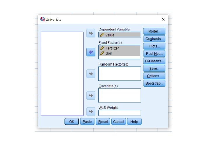
WORKED EXAMPLE 7. 5 A TWO WAY ANOVA ON PLANT ESTABLISHMENT IN DIFFERENT SUBSTRATES WITH AND WITHOUT FERTILISER APPLICATIONS: CALCULATION OF THE F STATISTICS Brick rubble Colliery spoil Brick rubble Fertilizer 비료 No Fertilizer Subsoil Similarly for Colliery spoil Subsoil test

Brick rubble Colliery spoil Fertilizer 비료 No Fertilizer Subsoil Similarly for Colliery spoil Subsoil test

Brick rubble Subsoil Colliery spoil Subsoil Fertilizer 비료 No Fertilizer Subsoil Similarly for Colliery spoil Subsoil test

WORKED EXAMPLE 7. 5 A TWO WAY ANOVA ON PLANT ESTABLISHMENT IN DIFFERENT SUBSTRATES WITH AND WITHOUT FERTILISER APPLICATIONS: CALCULATION OF THE F STATISTICS No Fertilizer
2 12 12")
Not in book Fmax Calculation Brick rubble Value Average (Value – Average)2 12 12 -11. 6=0. 4 0. 16 13 13 169 10 10 100 12 12 144 11 11 121 Average 11. 6 133. 54 534. 16 ----- = 133. 54 df (5 -1) 534. 16
2 11 11")
Not in book Fmax Calculation Colliery spoil Value Average (Value – Average)2 11 11 -10. 2=0. 8 0. 64 10 10 100 8 8 64 10 10 100 12 12 144 Average 10. 2 133. 54 107. 74 102. 16 70. 34 197. 14 408. 64 = ----- = 102. 16 df (5 -1)

Fmax Calculation Not in book Largest variance Fmax = ----------- Smallest variance 133. 54 Fmax = ------ = 1. 3 102. 16 133. 54 107. 74 102. 16 70. 34 197. 14 Fmax = ------ = 2. 80 70. 34 2. 8 Fmax = ------ = 2. 153 1. 3
")
Not in book Number of sample comparing = 6 Degrees of freedom (5 -1) = 4 Page 202 If the calculated value (2. 153 ) < table value 29. 5 Accept null hypothesis no significant difference Safe to proceed with the ANOVA

2 within 2 Application: With fertilizer & Without fertilizer 2 substrate total

2 total 2 interaction

Three F values obtained F values compared with df in critical value table Page 200 Table D. 7 Values calculated value of F for application is 4. 777 df of 1 and 24 Higher than table value P=0. 05 (4. 26), lower than P=0. 01 (7. 82), Therefore fertiliser application has a significant effect (P<0. 05)

Figure 7. 5 Effect of substrate and application of fertiliser on the number of plant species establishing. Bars represent standard errors Since all comparisons are significant, we conclude that: Subsoil>Brick rubble> Colliery spoil (at P=0. 05). The ANOVA results tell us that there is a significant effect of application.

Report There was a significant effect on the number of species establishing of both substrate type (F 2, 24=26. 64, P<0. 01) and fertiliser (F 1, 24=4. 78, P<0. 05), but no interaction (F 2, 24=0. 46, P>0. 05). Tukey’s multiple comparisons revealed that all three substrate types differed from each other, with subsoil supporting the most species, and colliery spoil supporting the least (P<0. 05). The addition of fertiliser increased the number of species on all three substrates.

Brick rubble With Fertilizer Colliery spoil Subsoil Without Fertilizer

There was a significant effect on the number of species establishing of both substrate type (F 2, 24=26. 64, P<0. 01) and fertiliser (F 1, 24=4. 78, P<0. 05), but no interaction (F 2, 24=0. 46, P>0. 05).

Page 157 Two-way ANOVA with single observations in each cell Single observations for each sample (i. e. there is only one data point for any combination of the two independent variables). Figure 7. 9 Visualising a two-way ANOVA with single observations in each cell Only one data point per sample Not possible to calculate the interaction Simple ANOVA Three types of variation: Column variable Row variable Independent variable.

WORKED EXAMPLE 7. 7 TWO-WAY ANOVA ON THE AMOUNT OF WATER ABSTRACTED (CUBIC METRES PER CAPITA PER ANNUM) FOR DIFFERENT PURPOSES ACROSS SIX REGIONS OF THE WORLD Data wrongly placed in book

Then SSabstraction and SSregion

Use SStotal SSabstraction & SSregion to calculate SSremainder

Degrees of freedom for abstraction purpose = 2 Degrees of freedom for remainder = 10 Table F value is 4. 10 Our value (F=1. 843) is lower than table value 4. 10 There is no significant effect of abstraction purpose Our value (F=1. 878) is lower than table value 4. 10 There is no significant effect of region

Table value for region degrees of freedom of 5 & remainder degrees of freedom of 10 is 3. 33 Out Statement: There is no significant difference in the quantities of water abstracted for each use (F 2, 10=1. 843, P>0. 05) and there are no significant differences between the quantity of water abstracted by the regions examined (F 5, 10=1. 878, P>0. 05).
- Slides: 68