7 Demand Forecasting in a Supply Chain Power

7 Demand Forecasting in a Supply Chain Power. Point presentation to accompany Chopra and Meindl Supply Chain Management, 5 e Copyright © 2013 Pearson Education, Inc. publishing as Prentice Hall. 1 -1 7 -1

Learning Objectives 1. Understand the role of forecasting for both an enterprise and a supply chain. 2. Identify the components of a demand forecast. 3. Forecast demand in a supply chain given historical demand data using time-series methodologies. 4. Analyze demand forecasts to estimate forecast error. Copyright © 2013 Pearson Education, Inc. publishing as Prentice Hall. 7 -2

Role of Forecasting in a Supply Chain • The basis for all planning decisions in a • supply chain Used for both push and pull processes – Production scheduling, inventory, aggregate planning – Sales force allocation, promotions, new production introduction – Plant/equipment investment, budgetary planning – Workforce planning, hiring, layoffs • All of these decisions are interrelated Copyright © 2013 Pearson Education, Inc. publishing as Prentice Hall. 7 -3

Characteristics of Forecasts 1. Forecasts are always inaccurate and should thus include both the expected value of the forecast and a measure of forecast error 2. Long-term forecasts are usually less accurate than short-term forecasts 3. Aggregate forecasts are usually more accurate than disaggregate forecasts 4. In general, the farther up the supply chain a company is, the greater is the distortion of information it receives Copyright © 2013 Pearson Education, Inc. publishing as Prentice Hall. 7 -4

Components and Methods • Companies must identify the factors that influence future demand then ascertain the relationship between these factors and future demand – – – Past demand Lead time of product replenishment Planned advertising or marketing efforts Planned price discounts State of the economy Actions that competitors have taken Copyright © 2013 Pearson Education, Inc. publishing as Prentice Hall. 7 -5

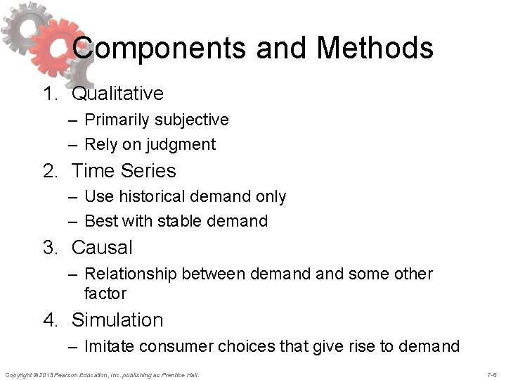
Components and Methods 1. Qualitative – Primarily subjective – Rely on judgment 2. Time Series – Use historical demand only – Best with stable demand 3. Causal – Relationship between demand some other factor 4. Simulation – Imitate consumer choices that give rise to demand Copyright © 2013 Pearson Education, Inc. publishing as Prentice Hall. 7 -6

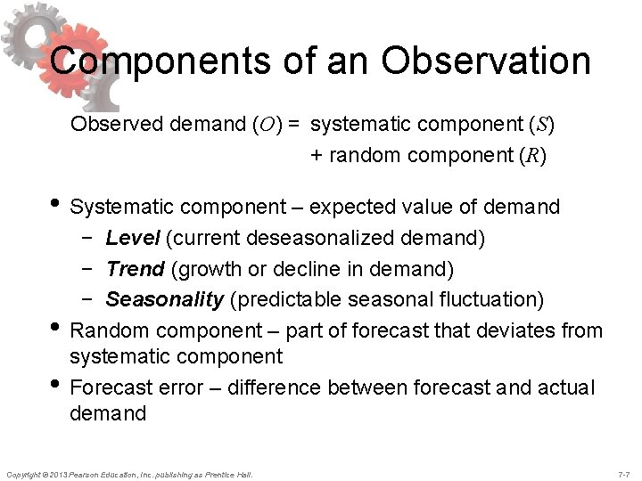
Components of an Observation Observed demand (O) = systematic component (S) + random component (R) • Systematic component – expected value of demand • • − Level (current deseasonalized demand) − Trend (growth or decline in demand) − Seasonality (predictable seasonal fluctuation) Random component – part of forecast that deviates from systematic component Forecast error – difference between forecast and actual demand Copyright © 2013 Pearson Education, Inc. publishing as Prentice Hall. 7 -7

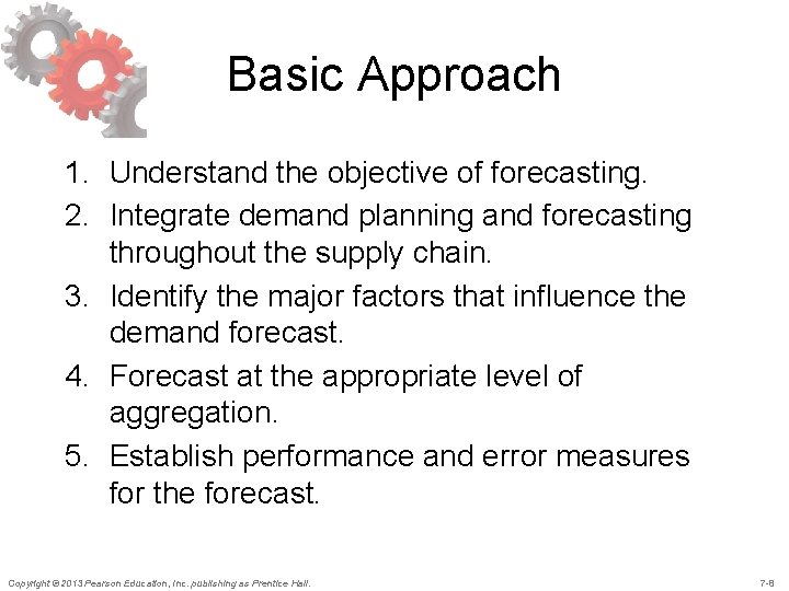
Basic Approach 1. Understand the objective of forecasting. 2. Integrate demand planning and forecasting throughout the supply chain. 3. Identify the major factors that influence the demand forecast. 4. Forecast at the appropriate level of aggregation. 5. Establish performance and error measures for the forecast. Copyright © 2013 Pearson Education, Inc. publishing as Prentice Hall. 7 -8

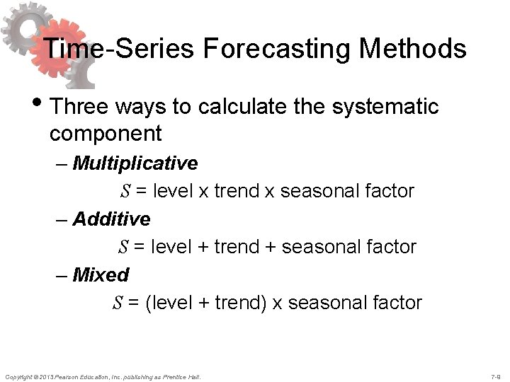
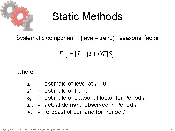
Time-Series Forecasting Methods • Three ways to calculate the systematic component – Multiplicative S = level x trend x seasonal factor – Additive S = level + trend + seasonal factor – Mixed S = (level + trend) x seasonal factor Copyright © 2013 Pearson Education, Inc. publishing as Prentice Hall. 7 -9

Static Methods where L T St Dt Ft = = = estimate of level at t = 0 estimate of trend estimate of seasonal factor for Period t actual demand observed in Period t forecast of demand for Period t Copyright © 2013 Pearson Education, Inc. publishing as Prentice Hall. 7 -10

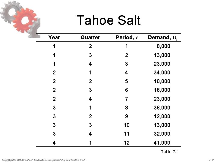
Tahoe Salt Year Quarter Period, t Demand, Dt 1 2 1 8, 000 1 3 2 13, 000 1 4 3 23, 000 2 1 4 34, 000 2 2 5 10, 000 2 3 6 18, 000 2 4 7 23, 000 3 1 8 38, 000 3 2 9 12, 000 3 3 10 13, 000 3 4 11 32, 000 4 1 12 41, 000 Table 7 -1 Copyright © 2013 Pearson Education, Inc. publishing as Prentice Hall. 7 -11

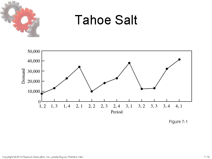
Tahoe Salt Figure 7 -1 Copyright © 2013 Pearson Education, Inc. publishing as Prentice Hall. 7 -12

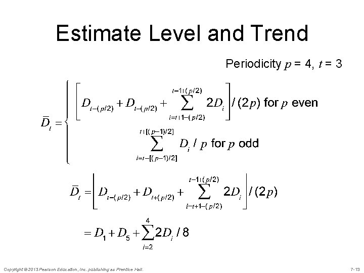
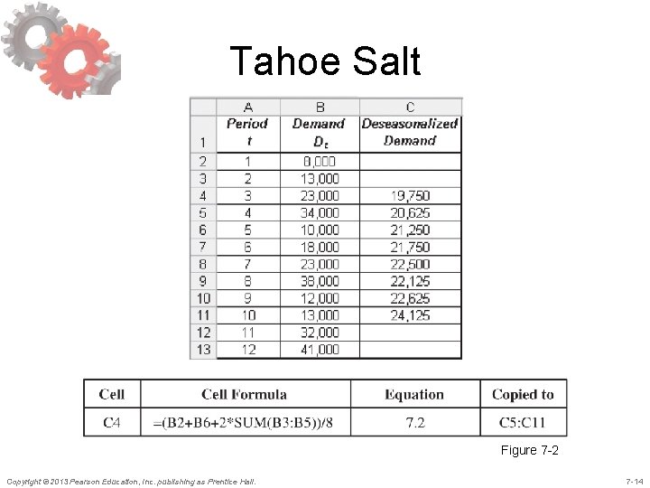
Estimate Level and Trend Periodicity p = 4, t = 3 Copyright © 2013 Pearson Education, Inc. publishing as Prentice Hall. 7 -13

Tahoe Salt Figure 7 -2 Copyright © 2013 Pearson Education, Inc. publishing as Prentice Hall. 7 -14

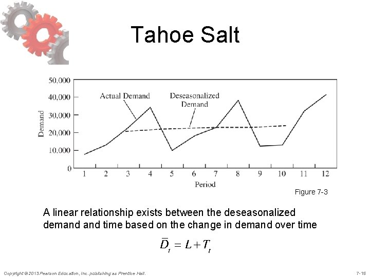
Tahoe Salt Figure 7 -3 A linear relationship exists between the deseasonalized demand time based on the change in demand over time Copyright © 2013 Pearson Education, Inc. publishing as Prentice Hall. 7 -15

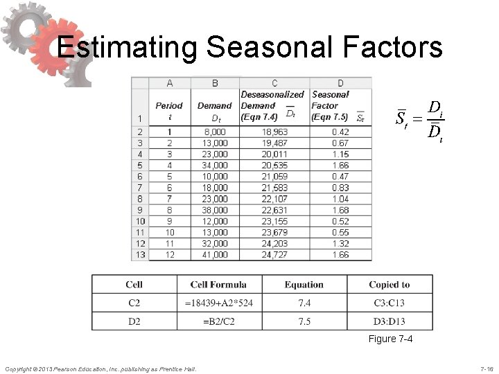
Estimating Seasonal Factors Figure 7 -4 Copyright © 2013 Pearson Education, Inc. publishing as Prentice Hall. 7 -16

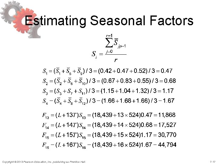
Estimating Seasonal Factors Copyright © 2013 Pearson Education, Inc. publishing as Prentice Hall. 7 -17

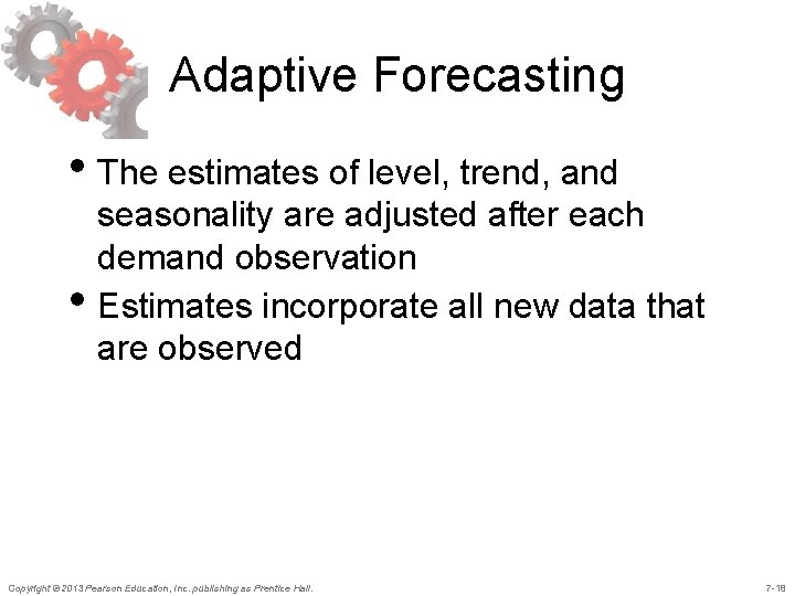
Adaptive Forecasting • The estimates of level, trend, and • seasonality are adjusted after each demand observation Estimates incorporate all new data that are observed Copyright © 2013 Pearson Education, Inc. publishing as Prentice Hall. 7 -18

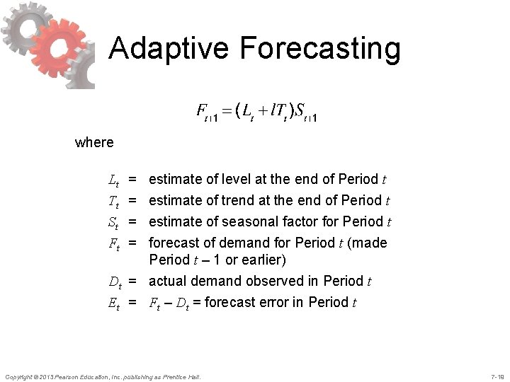
Adaptive Forecasting where estimate of level at the end of Period t estimate of trend at the end of Period t estimate of seasonal factor for Period t forecast of demand for Period t (made Period t – 1 or earlier) Dt = actual demand observed in Period t Et = Ft – Dt = forecast error in Period t Lt Tt St Ft = = Copyright © 2013 Pearson Education, Inc. publishing as Prentice Hall. 7 -19

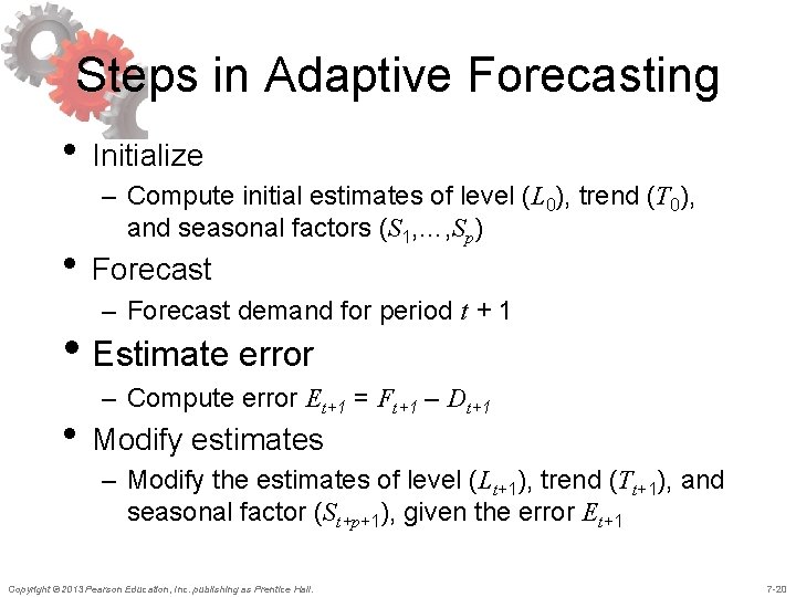
Steps in Adaptive Forecasting • Initialize – Compute initial estimates of level (L 0), trend (T 0), and seasonal factors (S 1, …, Sp) • Forecast – Forecast demand for period t + 1 • Estimate error – Compute error Et+1 = Ft+1 – Dt+1 • Modify estimates – Modify the estimates of level (Lt+1), trend (Tt+1), and seasonal factor (St+p+1), given the error Et+1 Copyright © 2013 Pearson Education, Inc. publishing as Prentice Hall. 7 -20

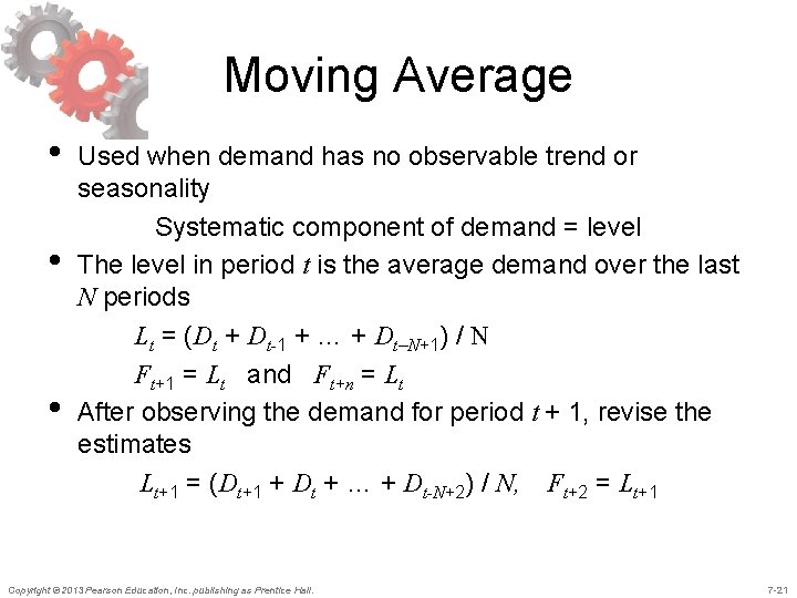
Moving Average • • • Used when demand has no observable trend or seasonality Systematic component of demand = level The level in period t is the average demand over the last N periods Lt = (Dt + Dt-1 + … + Dt–N+1) / N Ft+1 = Lt and Ft+n = Lt After observing the demand for period t + 1, revise the estimates Lt+1 = (Dt+1 + Dt + … + Dt-N+2) / N, Ft+2 = Lt+1 Copyright © 2013 Pearson Education, Inc. publishing as Prentice Hall. 7 -21

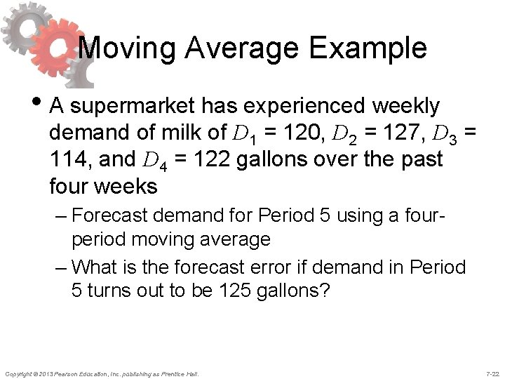
Moving Average Example • A supermarket has experienced weekly demand of milk of D 1 = 120, D 2 = 127, D 3 = 114, and D 4 = 122 gallons over the past four weeks – Forecast demand for Period 5 using a fourperiod moving average – What is the forecast error if demand in Period 5 turns out to be 125 gallons? Copyright © 2013 Pearson Education, Inc. publishing as Prentice Hall. 7 -22

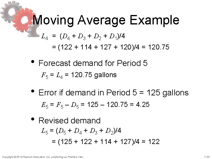
Moving Average Example L 4 = (D 4 + D 3 + D 2 + D 1)/4 = (122 + 114 + 127 + 120)/4 = 120. 75 • Forecast demand for Period 5 F 5 = L 4 = 120. 75 gallons • Error if demand in Period 5 = 125 gallons E 5 = F 5 – D 5 = 125 – 120. 75 = 4. 25 • Revised demand L 5 = (D 5 + D 4 + D 3 + D 2)/4 = (125 + 122 + 114 + 127)/4 = 122 Copyright © 2013 Pearson Education, Inc. publishing as Prentice Hall. 7 -23

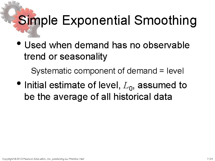
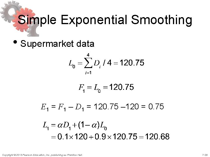
Simple Exponential Smoothing • Used when demand has no observable trend or seasonality Systematic component of demand = level • Initial estimate of level, L 0, assumed to be the average of all historical data Copyright © 2013 Pearson Education, Inc. publishing as Prentice Hall. 7 -24

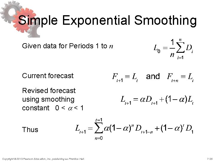
Simple Exponential Smoothing Given data for Periods 1 to n Current forecast Revised forecast using smoothing constant 0 < a < 1 Thus Copyright © 2013 Pearson Education, Inc. publishing as Prentice Hall. 7 -25

Simple Exponential Smoothing • Supermarket data E 1 = F 1 – D 1 = 120. 75 – 120 = 0. 75 Copyright © 2013 Pearson Education, Inc. publishing as Prentice Hall. 7 -26

Trend-Corrected Exponential Smoothing (Holt’s Model) • Appropriate when the demand is assumed to have a level and trend in the systematic component of demand but no seasonality Systematic component of demand = level + trend Copyright © 2013 Pearson Education, Inc. publishing as Prentice Hall. 7 -27

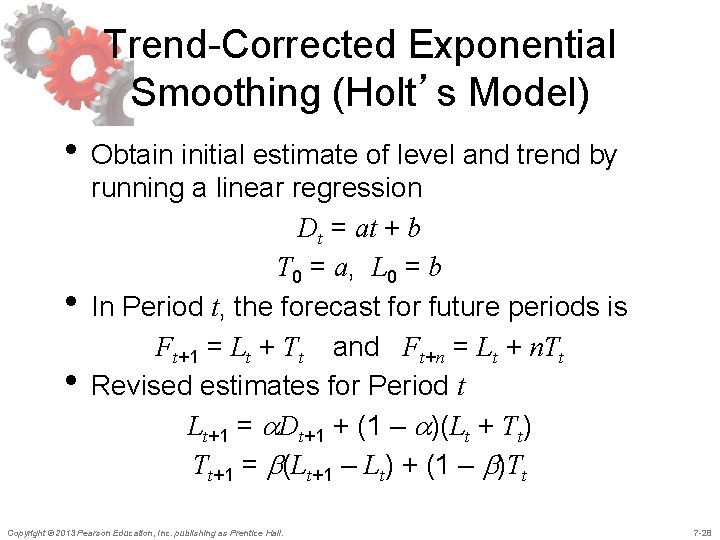
Trend-Corrected Exponential Smoothing (Holt’s Model) • Obtain initial estimate of level and trend by • • running a linear regression Dt = at + b T 0 = a, L 0 = b In Period t, the forecast for future periods is Ft+1 = Lt + Tt and Ft+n = Lt + n. Tt Revised estimates for Period t Lt+1 = a. Dt+1 + (1 – a)(Lt + Tt) Tt+1 = b(Lt+1 – Lt) + (1 – b)Tt Copyright © 2013 Pearson Education, Inc. publishing as Prentice Hall. 7 -28

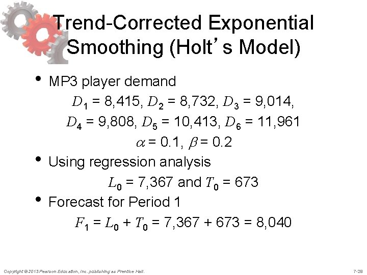
Trend-Corrected Exponential Smoothing (Holt’s Model) • MP 3 player demand • • D 1 = 8, 415, D 2 = 8, 732, D 3 = 9, 014, D 4 = 9, 808, D 5 = 10, 413, D 6 = 11, 961 a = 0. 1, b = 0. 2 Using regression analysis L 0 = 7, 367 and T 0 = 673 Forecast for Period 1 F 1 = L 0 + T 0 = 7, 367 + 673 = 8, 040 Copyright © 2013 Pearson Education, Inc. publishing as Prentice Hall. 7 -29

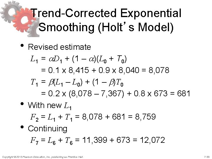
Trend-Corrected Exponential Smoothing (Holt’s Model) • Revised estimate • • L 1 = a. D 1 + (1 – a)(L 0 + T 0) = 0. 1 x 8, 415 + 0. 9 x 8, 040 = 8, 078 T 1 = b(L 1 – L 0) + (1 – b)T 0 = 0. 2 x (8, 078 – 7, 367) + 0. 8 x 673 = 681 With new L 1 F 2 = L 1 + T 1 = 8, 078 + 681 = 8, 759 Continuing F 7 = L 6 + T 6 = 11, 399 + 673 = 12, 072 Copyright © 2013 Pearson Education, Inc. publishing as Prentice Hall. 7 -30

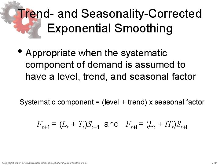
Trend- and Seasonality-Corrected Exponential Smoothing • Appropriate when the systematic component of demand is assumed to have a level, trend, and seasonal factor Systematic component = (level + trend) x seasonal factor Ft+1 = (Lt + Tt)St+1 and Ft+l = (Lt + l. Tt)St+l Copyright © 2013 Pearson Education, Inc. publishing as Prentice Hall. 7 -31

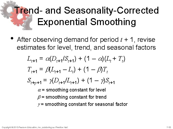
Trend- and Seasonality-Corrected Exponential Smoothing • After observing demand for period t + 1, revise estimates for level, trend, and seasonal factors Lt+1 = a(Dt+1/St+1) + (1 – a)(Lt + Tt) Tt+1 = b(Lt+1 – Lt) + (1 – b)Tt St+p+1 = g(Dt+1/Lt+1) + (1 – g)St+1 a = smoothing constant for level b = smoothing constant for trend g = smoothing constant for seasonal factor Copyright © 2013 Pearson Education, Inc. publishing as Prentice Hall. 7 -32

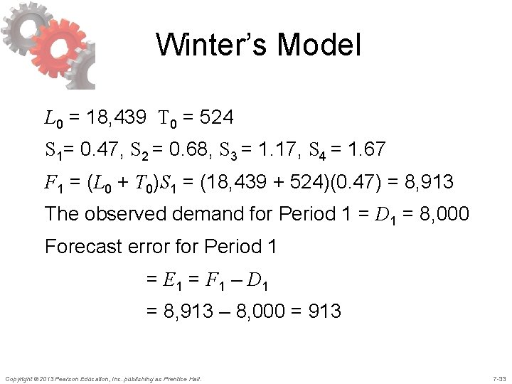
Winter’s Model L 0 = 18, 439 T 0 = 524 S 1= 0. 47, S 2 = 0. 68, S 3 = 1. 17, S 4 = 1. 67 F 1 = (L 0 + T 0)S 1 = (18, 439 + 524)(0. 47) = 8, 913 The observed demand for Period 1 = D 1 = 8, 000 Forecast error for Period 1 = E 1 = F 1 – D 1 = 8, 913 – 8, 000 = 913 Copyright © 2013 Pearson Education, Inc. publishing as Prentice Hall. 7 -33

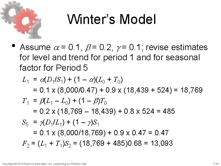
Winter’s Model • Assume a = 0. 1, b = 0. 2, g = 0. 1; revise estimates for level and trend for period 1 and for seasonal factor for Period 5 L 1 = a(D 1/S 1) + (1 – a)(L 0 + T 0) = 0. 1 x (8, 000/0. 47) + 0. 9 x (18, 439 + 524) = 18, 769 T 1 = b(L 1 – L 0) + (1 – b)T 0 = 0. 2 x (18, 769 – 18, 439) + 0. 8 x 524 = 485 S 5 = g(D 1/L 1) + (1 – g)S 1 = 0. 1 x (8, 000/18, 769) + 0. 9 x 0. 47 = 0. 47 F 2 = (L 1 + T 1)S 2 = (18, 769 + 485)0. 68 = 13, 093 Copyright © 2013 Pearson Education, Inc. publishing as Prentice Hall. 7 -34

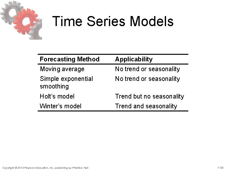
Time Series Models Forecasting Method Applicability Moving average No trend or seasonality Simple exponential smoothing No trend or seasonality Holt’s model Trend but no seasonality Winter’s model Trend and seasonality Copyright © 2013 Pearson Education, Inc. publishing as Prentice Hall. 7 -35

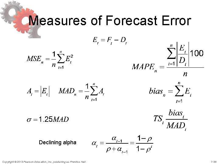
Measures of Forecast Error Declining alpha Copyright © 2013 Pearson Education, Inc. publishing as Prentice Hall. 7 -36

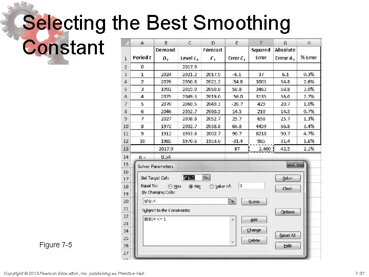
Selecting the Best Smoothing Constant Figure 7 -5 Copyright © 2013 Pearson Education, Inc. publishing as Prentice Hall. 7 -37

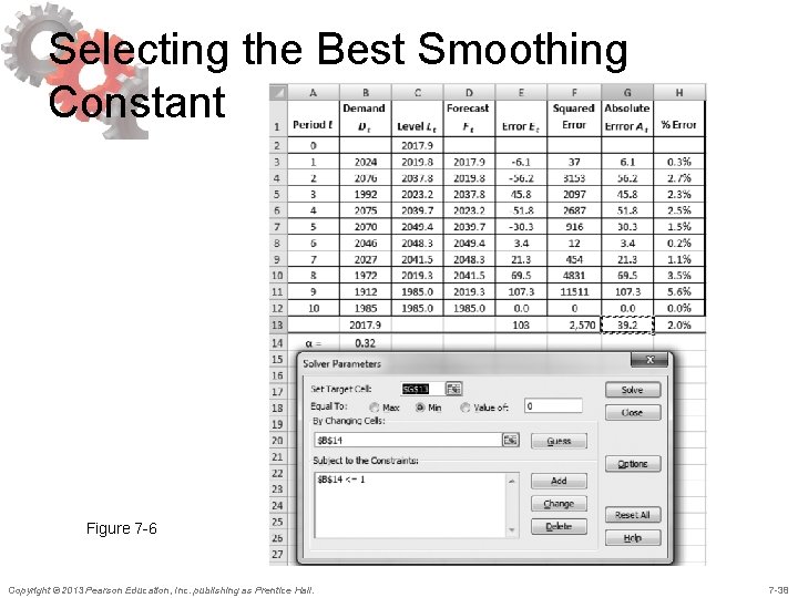
Selecting the Best Smoothing Constant Figure 7 -6 Copyright © 2013 Pearson Education, Inc. publishing as Prentice Hall. 7 -38

Forecasting Demand at Tahoe Salt • Moving average • Simple exponential smoothing • Trend-corrected exponential • smoothing Trend- and seasonality-corrected exponential smoothing Copyright © 2013 Pearson Education, Inc. publishing as Prentice Hall. 7 -39

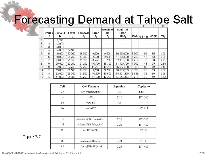
Forecasting Demand at Tahoe Salt Figure 7 -7 Copyright © 2013 Pearson Education, Inc. publishing as Prentice Hall. 7 -40

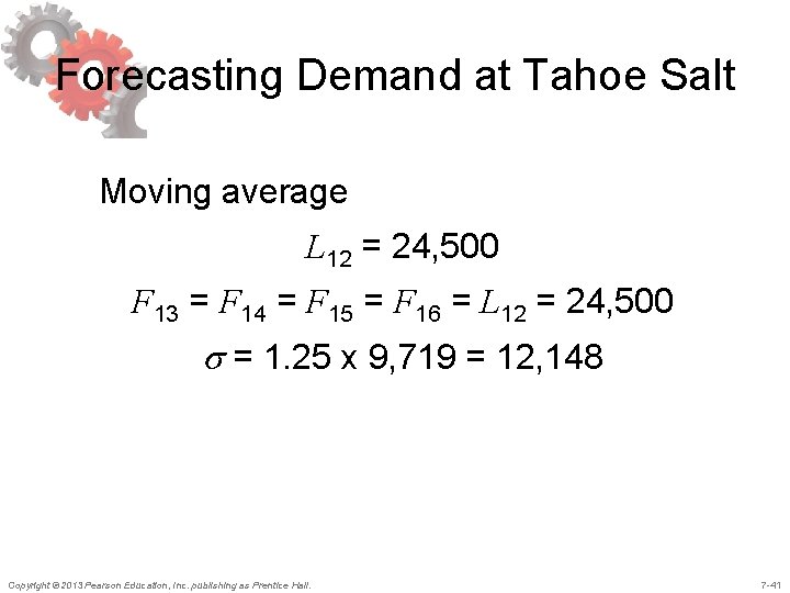
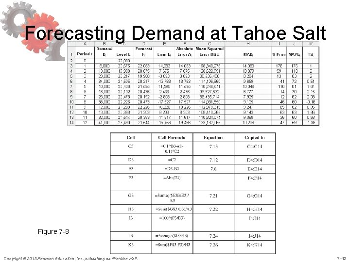
Forecasting Demand at Tahoe Salt Moving average L 12 = 24, 500 F 13 = F 14 = F 15 = F 16 = L 12 = 24, 500 s = 1. 25 x 9, 719 = 12, 148 Copyright © 2013 Pearson Education, Inc. publishing as Prentice Hall. 7 -41

Forecasting Demand at Tahoe Salt Figure 7 -8 Copyright © 2013 Pearson Education, Inc. publishing as Prentice Hall. 7 -42

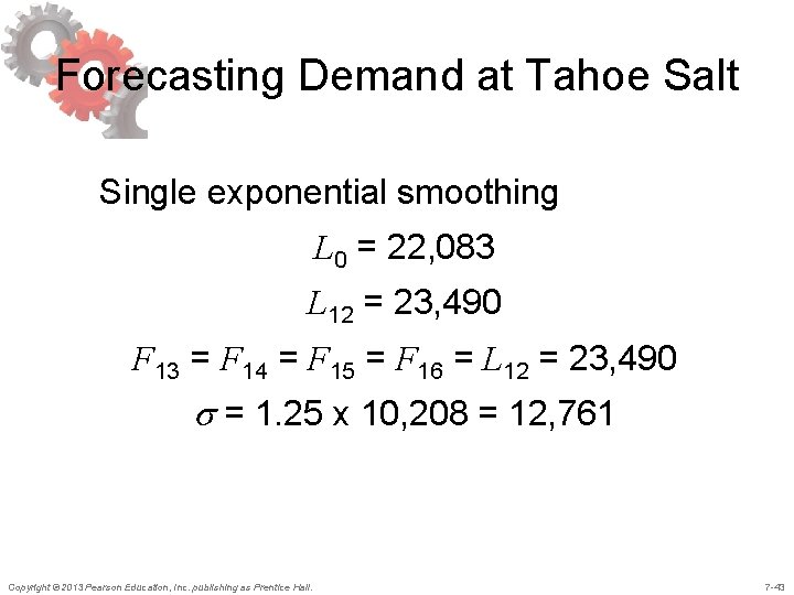
Forecasting Demand at Tahoe Salt Single exponential smoothing L 0 = 22, 083 L 12 = 23, 490 F 13 = F 14 = F 15 = F 16 = L 12 = 23, 490 s = 1. 25 x 10, 208 = 12, 761 Copyright © 2013 Pearson Education, Inc. publishing as Prentice Hall. 7 -43

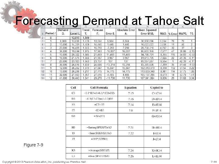
Forecasting Demand at Tahoe Salt Figure 7 -9 Copyright © 2013 Pearson Education, Inc. publishing as Prentice Hall. 7 -44

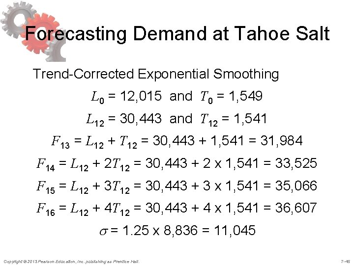
Forecasting Demand at Tahoe Salt Trend-Corrected Exponential Smoothing L 0 = 12, 015 and T 0 = 1, 549 L 12 = 30, 443 and T 12 = 1, 541 F 13 = L 12 + T 12 = 30, 443 + 1, 541 = 31, 984 F 14 = L 12 + 2 T 12 = 30, 443 + 2 x 1, 541 = 33, 525 F 15 = L 12 + 3 T 12 = 30, 443 + 3 x 1, 541 = 35, 066 F 16 = L 12 + 4 T 12 = 30, 443 + 4 x 1, 541 = 36, 607 s = 1. 25 x 8, 836 = 11, 045 Copyright © 2013 Pearson Education, Inc. publishing as Prentice Hall. 7 -45

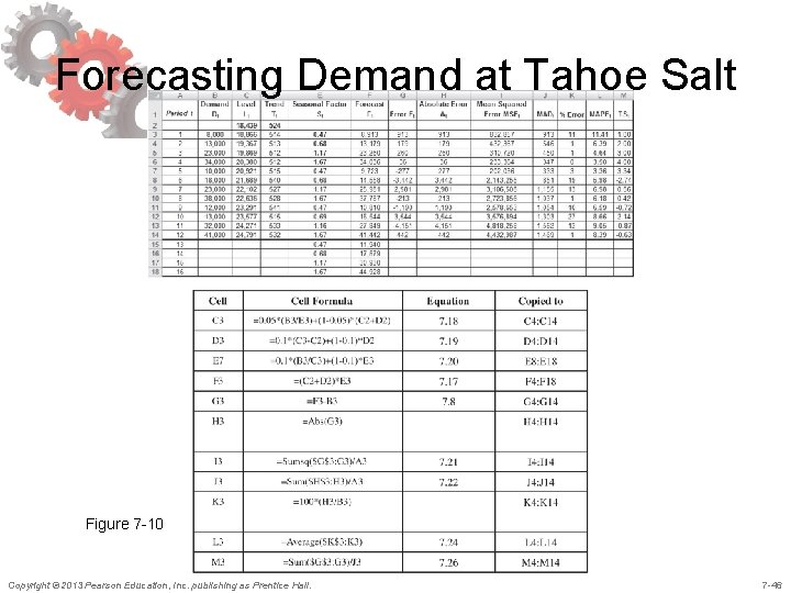
Forecasting Demand at Tahoe Salt Figure 7 -10 Copyright © 2013 Pearson Education, Inc. publishing as Prentice Hall. 7 -46

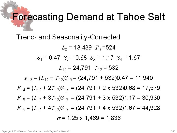
Forecasting Demand at Tahoe Salt Trend- and Seasonality-Corrected L 0 = 18, 439 T 0 =524 S 1 = 0. 47 S 2 = 0. 68 S 3 = 1. 17 S 4 = 1. 67 L 12 = 24, 791 T 12 = 532 F 13 = (L 12 + T 12)S 13 = (24, 791 + 532)0. 47 = 11, 940 F 14 = (L 12 + 2 T 12)S 13 = (24, 791 + 2 x 532)0. 68 = 17, 579 F 15 = (L 12 + 3 T 12)S 13 = (24, 791 + 3 x 532)1. 17 = 30, 930 F 16 = (L 12 + 4 T 12)S 13 = (24, 791 + 4 x 532)1. 67 = 44, 928 s = 1. 25 x 1, 469 = 1, 836 Copyright © 2013 Pearson Education, Inc. publishing as Prentice Hall. 7 -47

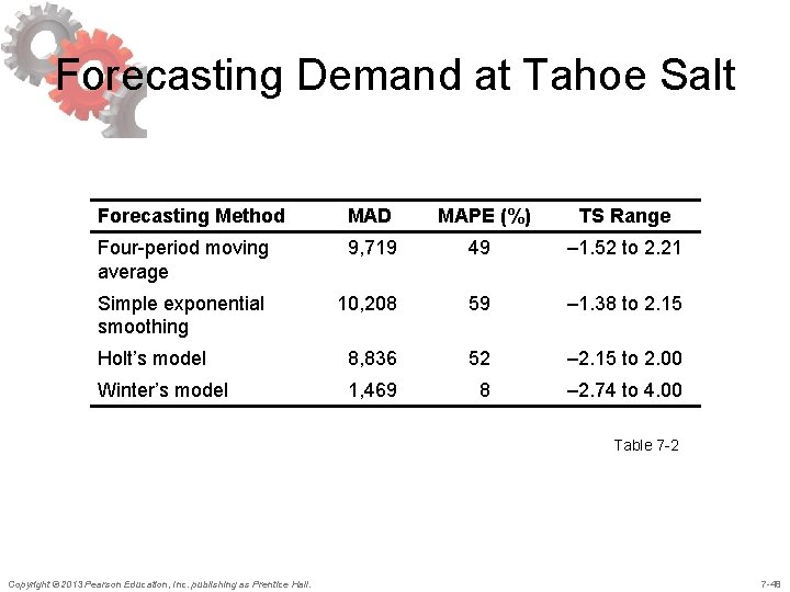
Forecasting Demand at Tahoe Salt Forecasting Method MAD MAPE (%) TS Range Four-period moving average 9, 719 49 – 1. 52 to 2. 21 Simple exponential smoothing 10, 208 59 – 1. 38 to 2. 15 Holt’s model 8, 836 52 – 2. 15 to 2. 00 Winter’s model 1, 469 8 – 2. 74 to 4. 00 Table 7 -2 Copyright © 2013 Pearson Education, Inc. publishing as Prentice Hall. 7 -48

The Role of IT in Forecasting • Forecasting module is core supply chain • • • software Can be used to best determine forecasting methods for the firm and by product categories and markets Real time updates help firms respond quickly to changes in marketplace Facilitate demand planning Copyright © 2013 Pearson Education, Inc. publishing as Prentice Hall. 7 -49

Risk Management • Errors in forecasting can cause significant • • misallocation of resources in inventory, facilities, transportation, sourcing, pricing, and information management Common factors are long lead times, seasonality, short product life cycles, few customers and lumpy demand, and when orders placed by intermediaries in a supply chain Mitigation strategies – increasing the responsiveness of the supply chain and utilizing opportunities for pooling of demand Copyright © 2013 Pearson Education, Inc. publishing as Prentice Hall. 7 -50

Forecasting In Practice • Collaborate in building forecasts • Share only the data that truly provide • value Be sure to distinguish between demand sales Copyright © 2013 Pearson Education, Inc. publishing as Prentice Hall. 7 -51

Summary of Learning Objectives 1. Understand the role of forecasting for both an enterprise and a supply chain 2. Identify the components of a demand forecast 3. Forecast demand in a supply chain given historical demand data using time-series methodologies 4. Analyze demand forecasts to estimate forecast error Copyright © 2013 Pearson Education, Inc. publishing as Prentice Hall. 7 -52

All rights reserved. No part of this publication may be reproduced, stored in a retrieval system, or transmitted, in any form or by any means, electronic, mechanical, photocopying, recording, or otherwise, without the prior written permission of the publisher. Printed in the United States of America. Copyright © 2013 Pearson Education, Inc. publishing as Prentice Hall. 7 -53