67535 Computer Games Programming Week 2 Randomness Perlin

67535: Computer Games Programming Week 2: Randomness: Perlin noise and Fractals Lighting: Phong-Blinn-Giraud; HDR Tutorial: Phong lighting in a fragment shader

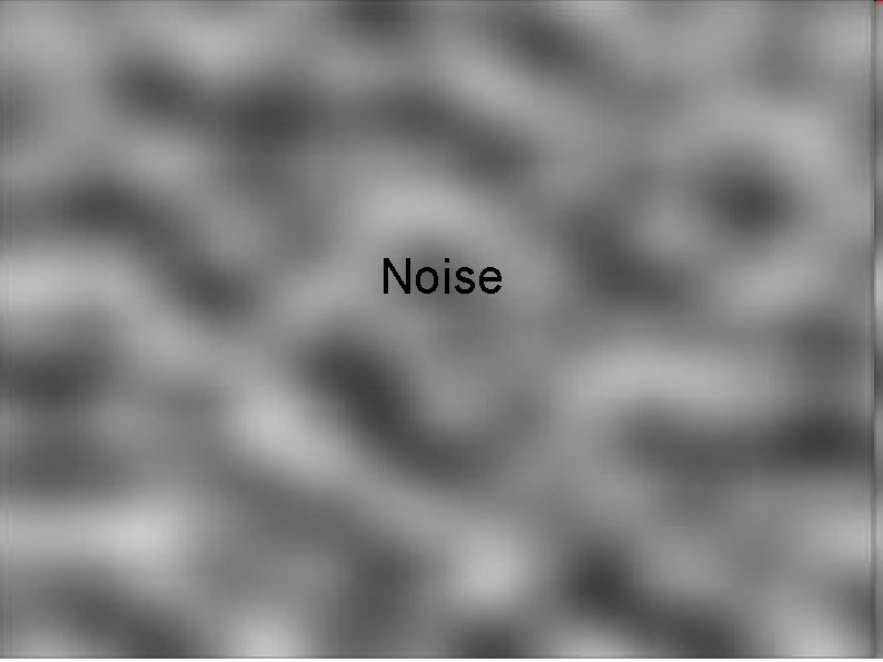
Noise

Noise and Procedural Modeling Create interest through difference Hide repeating patterns and artefacts from other generation methods (e. g. faulting) Can be used as a basis function for fractals Noise is like salt: adds flavour to procedural content

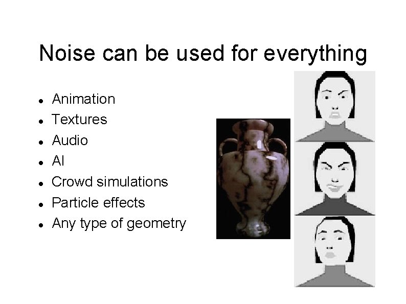
Noise can be used for everything Animation Textures Audio AI Crowd simulations Particle effects Any type of geometry

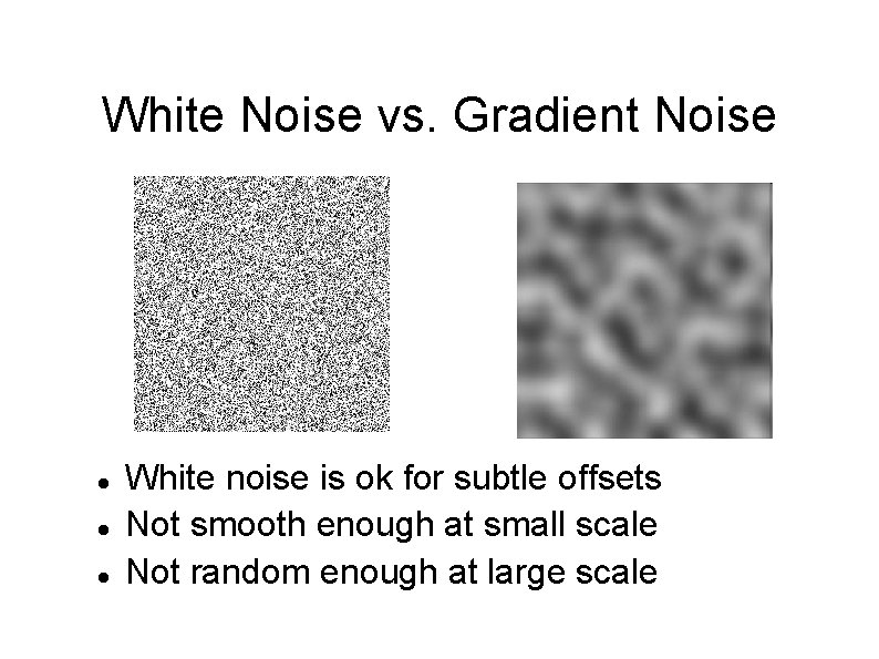
White Noise vs. Gradient Noise White noise is ok for subtle offsets Not smooth enough at small scale Not random enough at large scale

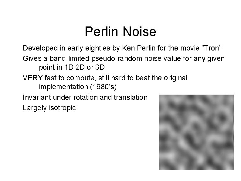
Perlin Noise Developed in early eighties by Ken Perlin for the movie “Tron” Gives a band-limited pseudo-random noise value for any given point in 1 D 2 D or 3 D VERY fast to compute, still hard to beat the original implementation (1980’s) Invariant under rotation and translation Largely isotropic

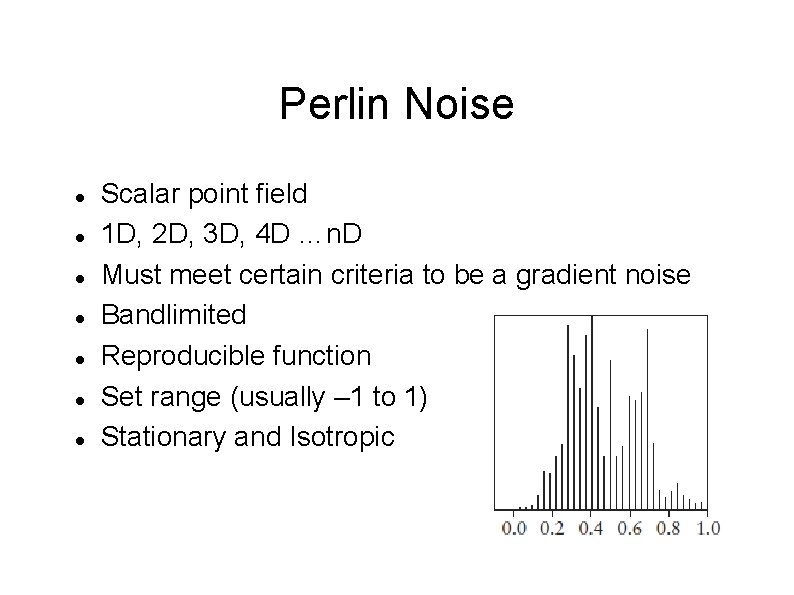
Perlin Noise Scalar point field 1 D, 2 D, 3 D, 4 D …n. D Must meet certain criteria to be a gradient noise Bandlimited Reproducible function Set range (usually – 1 to 1) Stationary and Isotropic

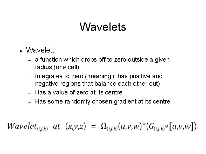
Perlin Noise A gradient noise - uses a set of pseudo-random gradients at regularly spaced points and interpolate between (blending function) Overview: Space divided into regular lattice One pseudo-random wavelet per lattice point (or per side of cubical cell) Scalar value of function = Sum of wavelets

Wavelets Wavelet: a function which drops off to zero outside a given radius (one cell) Integrates to zero (meaning it has positive and negative regions that balance each other out) Has a value of zero at its centre Has some randomly chosen gradient at its centre

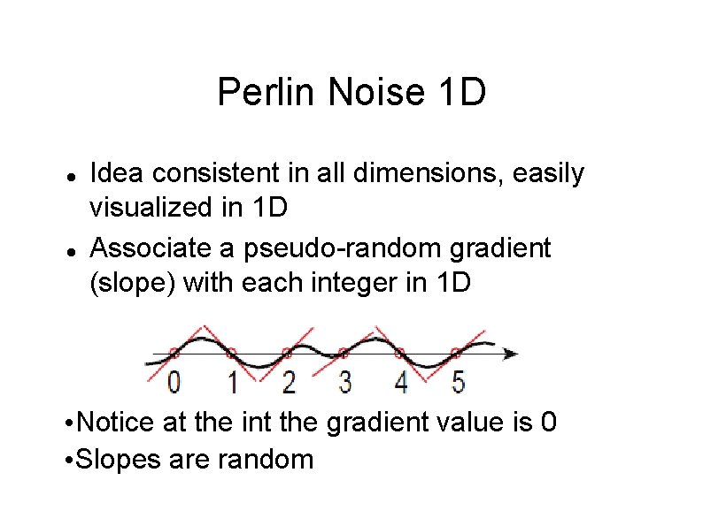
Perlin Noise 1 D Idea consistent in all dimensions, easily visualized in 1 D Associate a pseudo-random gradient (slope) with each integer in 1 D • Notice at the int the gradient value is 0 • Slopes are random

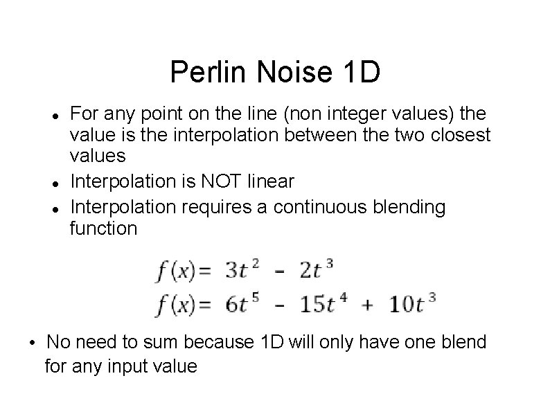
Perlin Noise 1 D For any point on the line (non integer values) the value is the interpolation between the two closest values Interpolation is NOT linear Interpolation requires a continuous blending function • No need to sum because 1 D will only have one blend for any input value

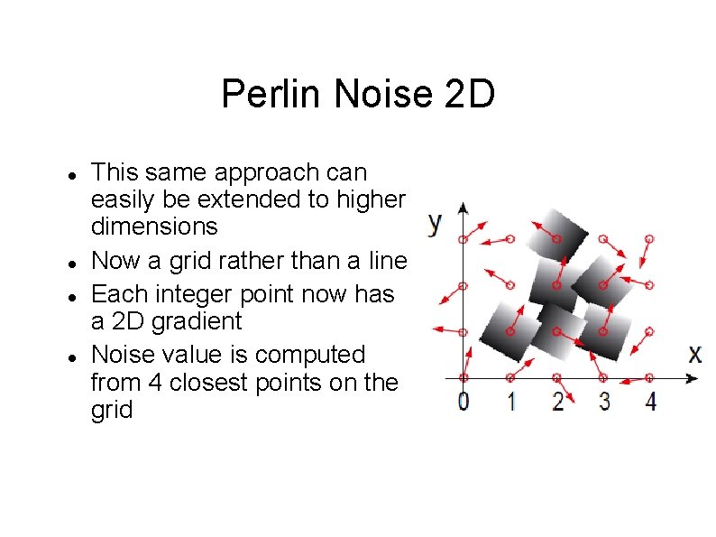
Perlin Noise 2 D This same approach can easily be extended to higher dimensions Now a grid rather than a line Each integer point now has a 2 D gradient Noise value is computed from 4 closest points on the grid

Perlin Noise 2 D For 2 D (and higher dimensions), we need to sum up the contributions of each wavelet. Still use the blending function (spline) For 2 D use a bilinear interpolation First interpolate in the x, then in the y using the results from the x Easily extends to 3 D, 4 D, …, n. D

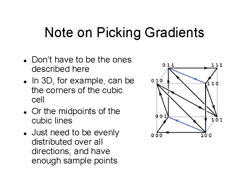
Note on Picking Gradients Don’t have to be the ones described here In 3 D, for example, can be the corners of the cubic cell Or the midpoints of the cubic lines Just need to be evenly distributed over all directions, and have enough sample points

Perlin Noise Algorithm Summary Compute which cubical “cell” we are in Compute the wavelet centred on each of the surrounding sides of the cube Sum the wavelets Look at Procedural Modelling book and the Gustavson’s paper for implementation details

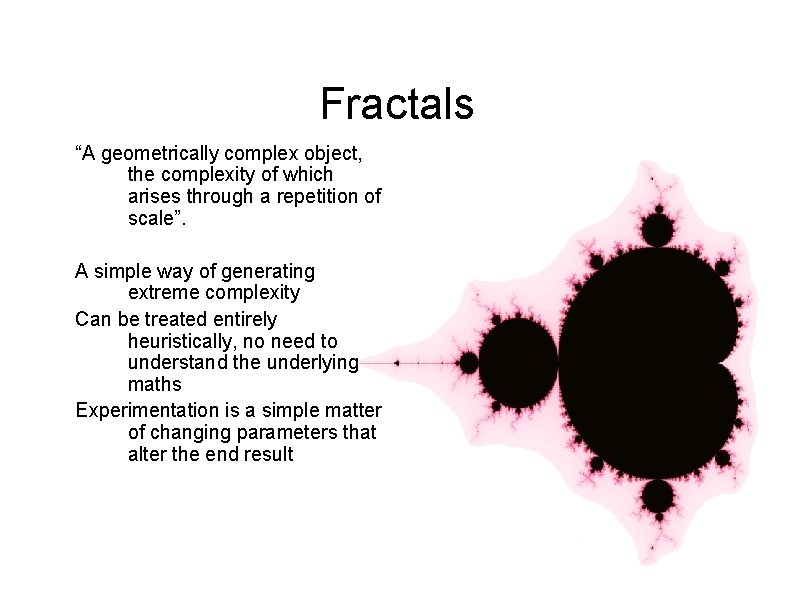
Fractals “A geometrically complex object, the complexity of which arises through a repetition of scale”. A simple way of generating extreme complexity Can be treated entirely heuristically, no need to understand the underlying maths Experimentation is a simple matter of changing parameters that alter the end result

Basis Function Fractals rely on repetition over scale Something must be repeated Technically anything can be used, but it is better if it’s: Controllable Self Similar Deterministic Easy to calculate

Fractals Use a variant of Perlin noise (absolute value, squared, etc) as a basis function How the basis function is rescaled and combined (through addition, multiplication, subtraction) determines the properties of the fractal Octaves indicate the dimensionality and fractional values can be extremely useful for continuous level of detail schemes

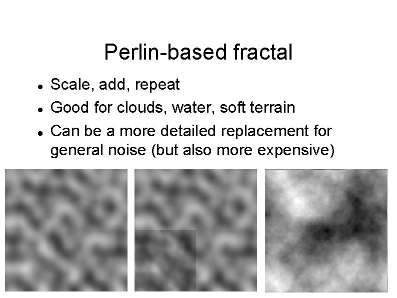
Perlin-based fractal Scale, add, repeat Good for clouds, water, soft terrain Can be a more detailed replacement for general noise (but also more expensive)

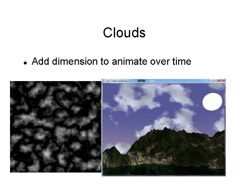
Clouds Add dimension to animate over time

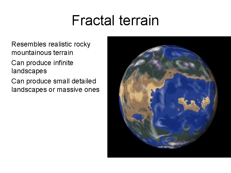
Fractal terrain Resembles realistic rocky mountainous terrain Can produce infinite landscapes Can produce small detailed landscapes or massive ones

Multifractals Extends on homogenous fractals and blends two or more fractal functions together to create objects that exhibit a blend of features For example change the blend ratio over the height of the basis function to give sharp mountains, but soft hills and lowlands

Reading on Procedural Content Generation Games Programming Gems 1 & 2 Texturing and Modelling : A Procedural Approach Perlin: http: //www. noisemachine. com/talk 1/index. html http: //http. developer. nvidia. com/GPUGems 2/gpugems 2_cha pter 26. html Musgrave: http: //www. ypoart. com/downloads/Musgrave. htm http: //pcg. wikidot. com/ http: //www. pandromeda. com/ http: //www. planetside. co. uk/terragen/ algorithmicbotany. org/papers/abop. pdf

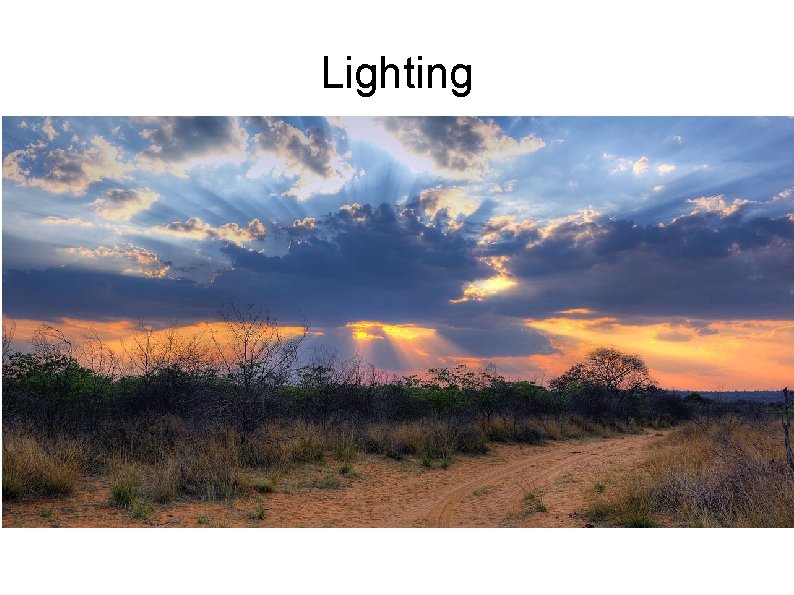
Lighting

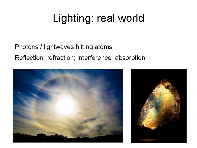
Lighting: real world Photons / lightwaves hitting atoms Reflection; refraction; interference; absorption…

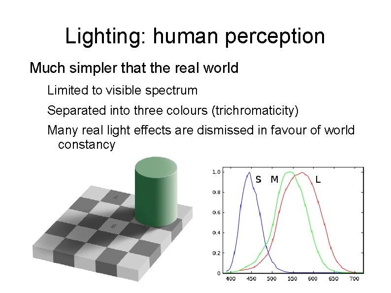
Lighting: human perception Much simpler that the real world Limited to visible spectrum Separated into three colours (trichromaticity) Many real light effects are dismissed in favour of world constancy

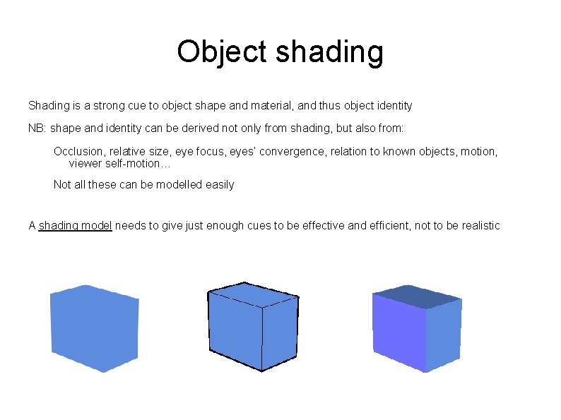
Object shading Shading is a strong cue to object shape and material, and thus object identity NB: shape and identity can be derived not only from shading, but also from: Occlusion, relative size, eye focus, eyes’ convergence, relation to known objects, motion, viewer self-motion… Not all these can be modelled easily A shading model needs to give just enough cues to be effective and efficient, not to be realistic

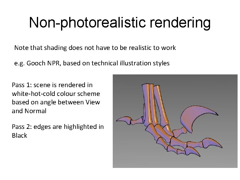
Non-photorealistic rendering Note that shading does not have to be realistic to work e. g. Gooch NPR, based on technical illustration styles Pass 1: scene is rendered in white-hot-cold colour scheme based on angle between View and Normal Pass 2: edges are highlighted in Black

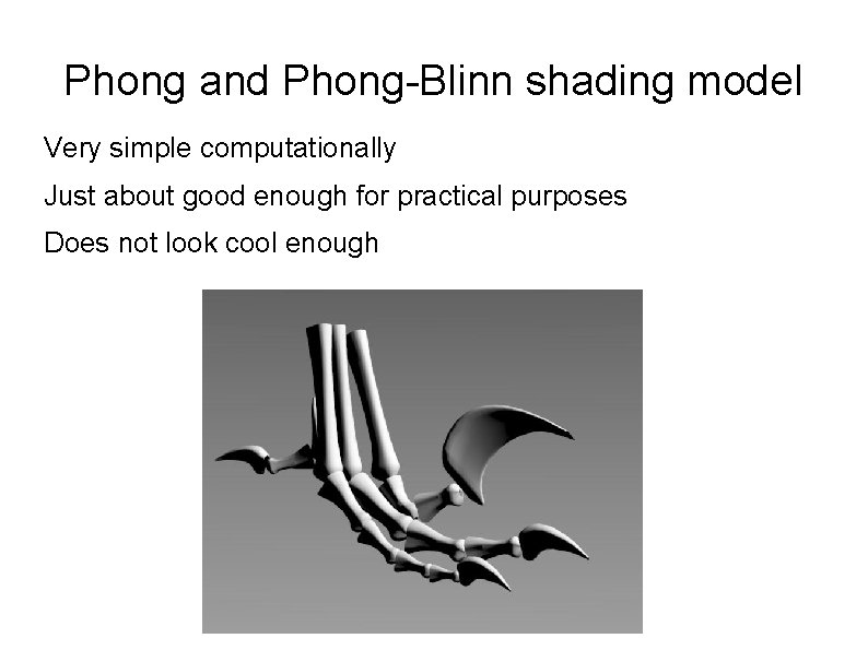
Phong and Phong-Blinn shading model Very simple computationally Just about good enough for practical purposes Does not look cool enough

Phong Bui-tuong (1975) The most common reflection model in CG An acceptable compromise between simplicity and accuracy Largely empirical Local reflection model – does not handle global effects of light reflecting between surfaces

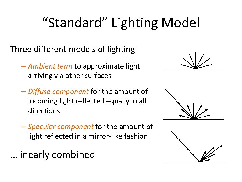
“Standard” Lighting Model Three different models of lighting – Ambient term to approximate light arriving via other surfaces – Diffuse component for the amount of incoming light reflected equally in all directions – Specular component for the amount of light reflected in a mirror-like fashion …linearly combined

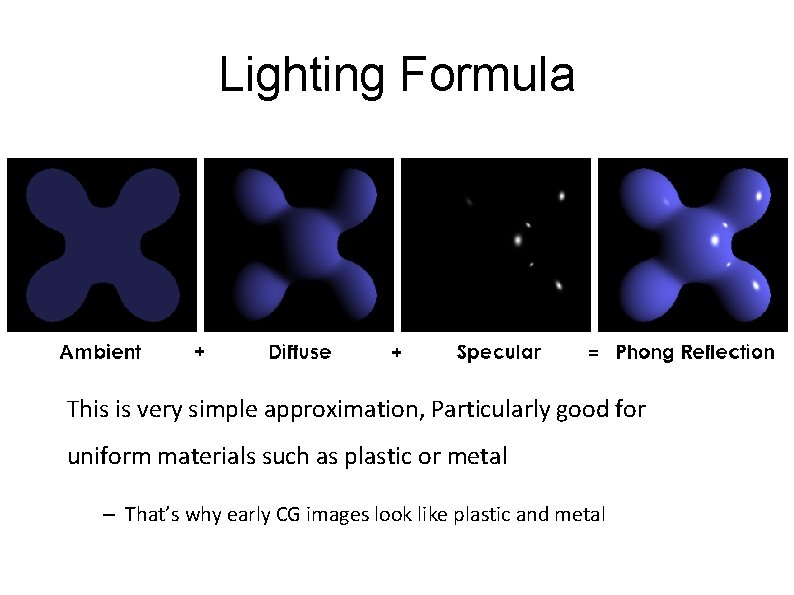
Lighting Formula This is very simple approximation, Particularly good for uniform materials such as plastic or metal – That’s why early CG images look like plastic and metal

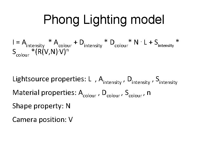
Phong Lighting model I = Aintensity * Acolour + Dintensity * Dcolour* N. L + Sintensity * Scolour *(R(V, N). V)n Lightsource properties: L , Aintensity , Dintensity , Sintensity Material properties: Acolour , Dcolour , Scolour , n Shape property: N Camera position: V

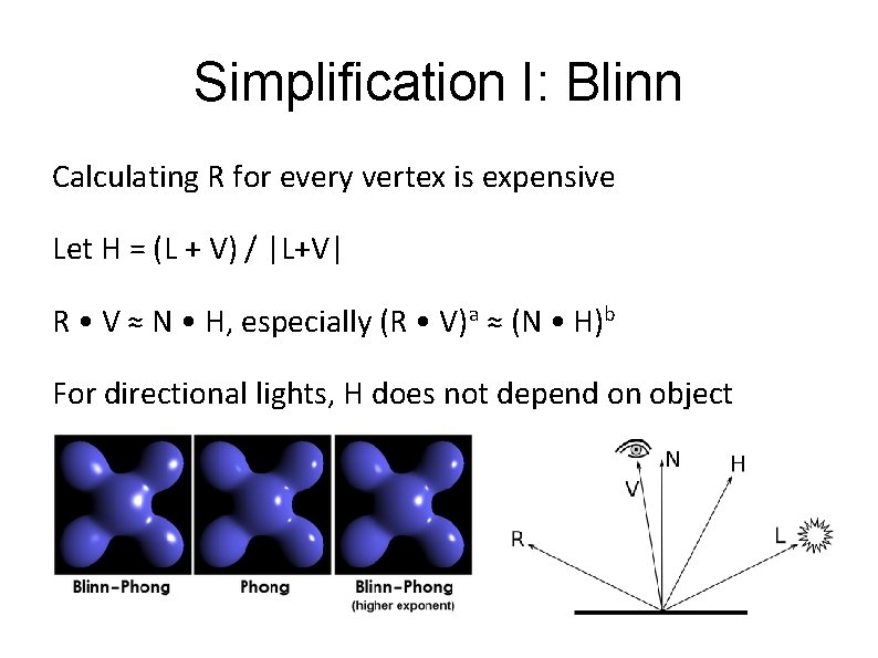
Simplification I: Blinn Calculating R for every vertex is expensive Let H = (L + V) / |L+V| R • V ≈ N • H, especially (R • V)a ≈ (N • H)b For directional lights, H does not depend on object

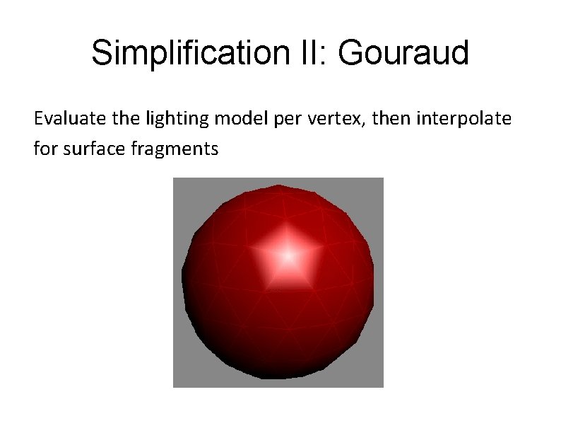
Simplification II: Gouraud Evaluate the lighting model per vertex, then interpolate for surface fragments

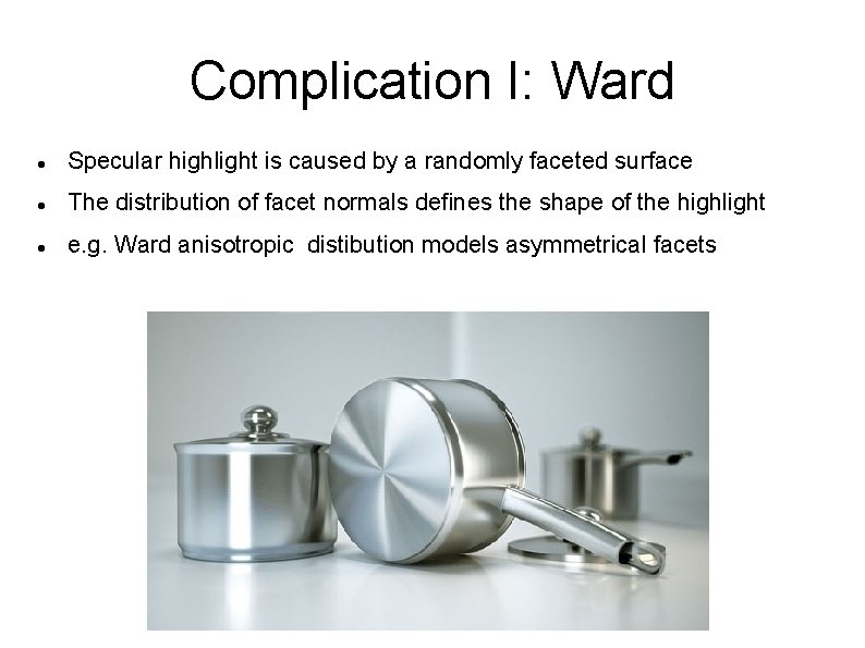
Complication I: Ward Specular highlight is caused by a randomly faceted surface The distribution of facet normals defines the shape of the highlight e. g. Ward anisotropic distibution models asymmetrical facets

NB: Lighting space Face normals, light direction and camera positions must be in the same space In order to get the normals correctly specified in world or view space, we would multiply by world or view matrix – This does not preserve scaling – Need to use inverse-transposed world or view matrix – In most practical cases, inverse-transpose is equal to the matrix

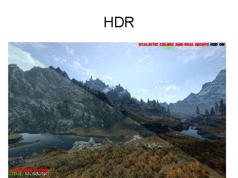
HDR

Dynamic Range Dynamic range is the ratio between the largest and smallest possible values of a changeable quantity DR of an image is the ratio of brightness of the lightest and the darkest pixel; a measure of image contrast DR of a display is a ratio of brightness of the lightest and the darkest image the display can produce (full black to full white) DR of human eye at any given time: 1: 10, 000; overall (with accommodation): 1: 1, 000 DR of a good digital camera: 1: 10, 000 DR of an LCD display: 1: 500 to 1: 1, 000 DR of a RGB colour space: 1: 256

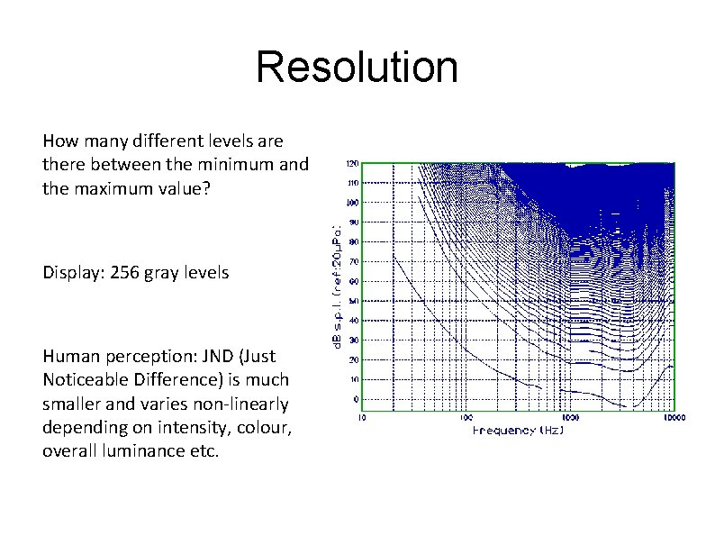
Resolution How many different levels are there between the minimum and the maximum value? Display: 256 gray levels Human perception: JND (Just Noticeable Difference) is much smaller and varies non-linearly depending on intensity, colour, overall luminance etc.

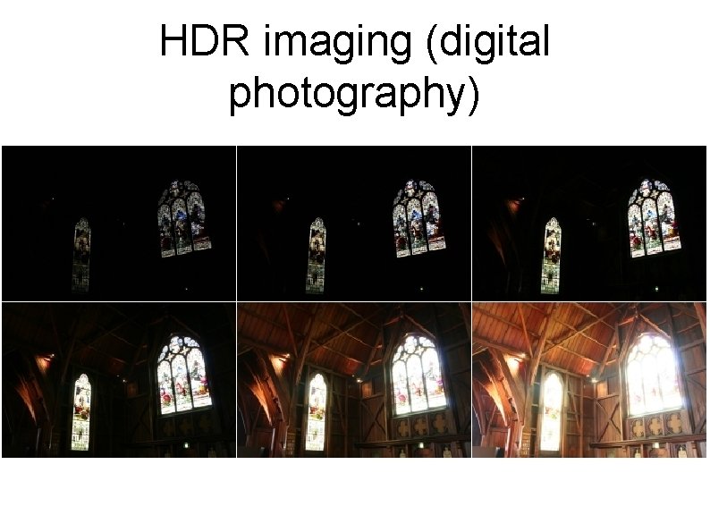
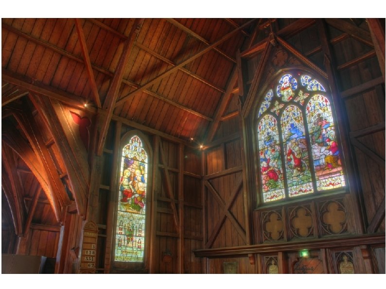
HDR imaging (digital photography)

HDR rendering Light calculations are done in high resolution and dynamic range – Float: DR of 1: 65, 536 Resulting brightness value of a pixel is translated to display DR as late as possible (i. e. pixel shader at the last stage of postprocessing) Non-linear mapping functions (e. g. Sigmoids) Local tone-mapping (preserving local contrast)

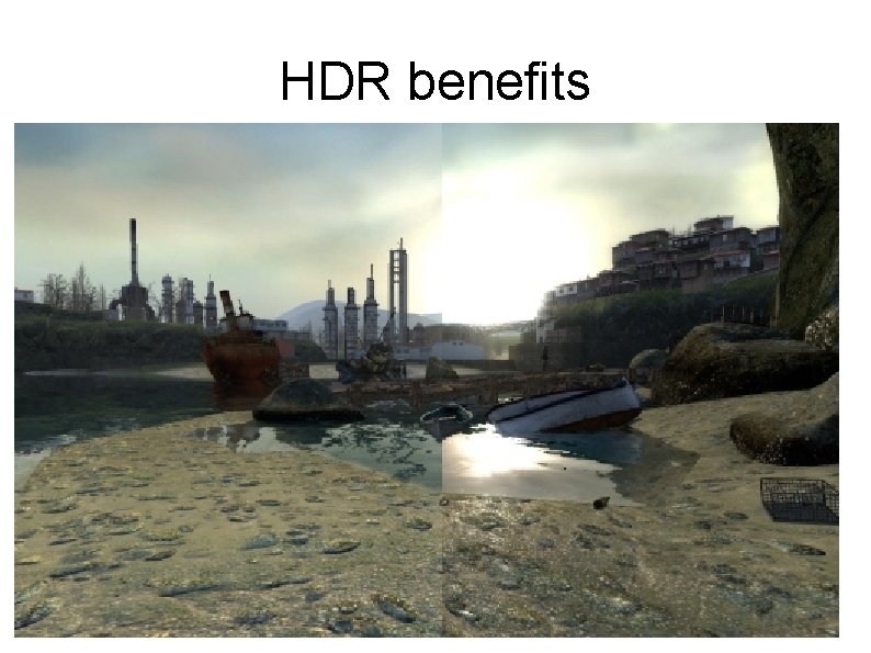
HDR benefits