67535 Computer Games Programming Textures PostProcessing Texture mapping

67535: Computer Games Programming Textures & Post-Processing

Texture mapping Motivation: adjusting colour (and other parameters) per fragment, not per vertex Solution: texturing each face from an image

Texture issues Min/Mag filters Antialiasing Mip-maps Coordinate overflow

Fragment shaders and textures Fragment shaders receive sets of texture coordinates and combine values sampled from textures (texels) The trick is to use textures as generic per-fragment data structures, not just for colour Vertex data Position (x, y, z, w) Texture coordinates (u, v) Normal to face (nx, ny, nz)

Case study 1: reflexion mapping

Skybox An infinitely faraway sphere with a cube map texture Cube map: special texture data structure; six square 2 D textures on the faces of a cube; each face is a scene from a 90° field of view camera placed at the origin looking along an axis

Cube Map coordinates +T, +Y +S, +X -R, -Z

Reflections of Skybox angle of incidence = angle of reflection Vertex shader outputs a texture coordinate which is the “reflection” of the vector from camera to object Fragment shader maps that texture coordinate into a skybox

Refractions of Skybox Same as reflection, only instead of reflecting, the view vector is changed according to Snell’s law: ni sin (i) = nr sin (r) Where i is angle of incidence, r is angle of refraction, ni and nr are the refractive indices of the two mediums Sample refractive indices: Air = 1. 00; water = 1. 33; Diamond = 2. 42

Glass Linear combination of reflexion and refraction based on angle from camera

Limitations

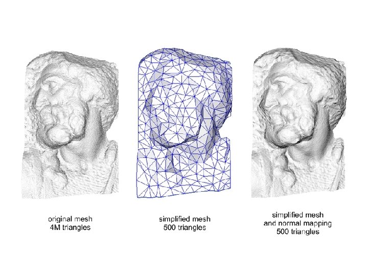
Case study 2: bump mapping

Motivation Phong lighting is good for smooth objects – What about high frequency details such as crevices, bumps or scratches? Increasing poly count is costly – Makes no sense for large distances when high detail level is not required Need different level of detail at different distances – mip-mapping, but for detail, not colour

General idea Separate objects into low-poly shape and variable levels of detail Geometry (polygons) encodes shape ‘Texture’ encodes fine detail – not colour

Displacement mapping Modifying the mesh – Requires tessellation or on-the -fly mesh generation capabilities – Accurate but slow

Bump mapping Perturb the surface normal used in the lighting calculations – Real surface geometry is unchanged – But there is an appearance of bumpiness Simplest to implement and compute Does not affect silhouette, occlusion, shadows etc

Implementations Blinn bump mapping – Texture encodes height of texel above the face – Fragment normal is calculated at runtime Normal mapping – Texture encodes dn - normal vector displacement relative to face normal – pre-computed from height map at design stage

Tangent space (TBN) • Aka Texture space or polygon face space – T tangent, tangent to surface – B binormal, ‘the other tangent to surface’ – N normal, normal to surface

Vertex shader 1. Compute TBN-base for each triangle of mesh 2. Transform the light vector from object space to tangent space 3. Output light vector in tangent space Fragment shader 1. Use light vector and normal displacement (from texture) to calculate shading

Limitations

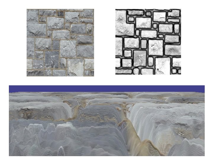
Parallax mapping (2001) Using height-map and angle from surface to viewer to displace the texture coordinates – Simple and fast, yet almost as good-looking as displacement mapping – Improvements for occlusions and self-shadows

No parallax mapping

With Parallax mapping

Relief mapping Several layers of heightmaps and normals stored for each texel Describes ‘mesostructure’

Post-Processing

Post processing idea • Render to off-screen buffer • Apply various Im. Pr techniques to that buffer • Render it as a texture on a quad – Quad that fills all the screen –. . . or not

Im. Pr in a small nutshell Image processing for post-processing – not for image analysis, surveillance, photoshop etc. Noise reduction Object identification Compression

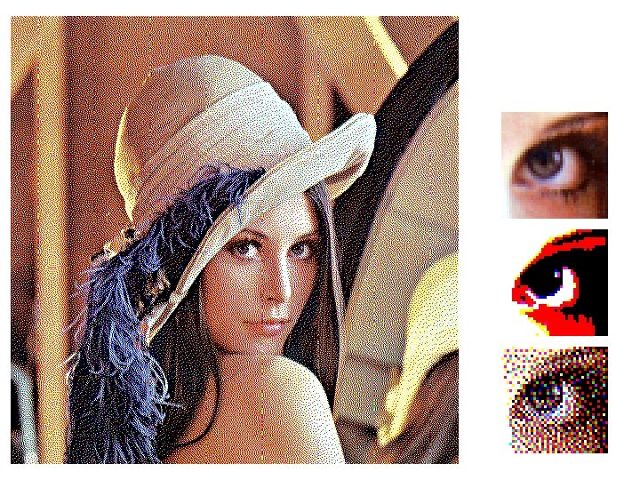
Offtopic: Lenna Standard testing image in Image Processing Model: Lena Sjooblom Origin: 1972 Playboy “a nice mixture of detail, flat regions, shading, and texture” more history: www. lenna. org

Types of image operations Per-pixel operations 1 – calculate an output pixel value from an input pixel value – using a look-up table (LUT) or a function Linear operations – matrix additions/multiplications etc. Non-linear operations – Convolutions – Frequency domain operations 0 input pixel value 1

Brightness out = in*0. 5+0. 5

Contrast out = in*0. 3+0. 3 out = in*1. 5 Problem: clamping

Gamma correction γ =1

Inversion, colour reduction out = 1 -in out = round(in) out =floor(in*4. 99)/5

Better colour reduction: Dithering Colour reduction is too coarse Solution: error propagation for every pixel (left to right and top to bottom) 1. out = floor(in*N*0. 999)/N 2. error = in – out 3. spread the error to pixels on the right and bottom Different weights of error spread lead to different results; Floyd-Steinberd weights are the accepted best

Non-uniform pixel-area ops Using neighbouring pixels based on input pixel position Cannot be done with convolution, easy with shaders Can be iterated for stronger effect From http: //www. jhlabs. com/ip/blurring. html

Convolution

Image convolution Discrete, finite, 2 D Input: A[ma, na], B[mb, nb] Output: conv[ma+mb, na+nb] for ia = 1: ma for jb = 1: na conv[ia, ja] = 0 for ib = 1: mb for jb = 1: nb conv[ia, ja] += A[ia, ja]*B[ia+ib, ja+jb]

Properties of convolution Commutative f*h(x) = h*f(x) Associative f*(h*g)(x) = (f*h)*g(x) Distributive over addition f*(h + g)(x) = (f*h)(x)+(f*g)(x) Proofs: http: //www. cs. dartmouth. edu/farid/tutorials/fip. pdf

Problems: edges and bounds • Solution: – clamping – scaling – designing filters that add up to 1 – Scaling whatever filter you have to add up to 1

Problem: complexity Solution 1: decomposition into smaller matrices. If F can be decomposed into F=f 1*f 2 then G*F = G*(f 1*f 2) = (G*f 1)*f 2 Solution 2: use Fast Fourier Transform

Image + filters Convolution of (large) image matrix with several small filter matrices – fast to calculate – small edges – filters can be designed to preserve data in a required range

Convolution kernels A kernel defines the operation to be performed in the area around the input pixel to calculate the value of the output pixel For efficiency reasons: – Kernels are made as small as possible – Large kernels are decomposed into a series of small ones, if at all possible – E. g. Gaussian blur is a repeated convolution of horizontal [½ ½] and vertical [½ ½]’

Blur 1/9 1/9 1/9 1 2 4 2 1 1 1 2 1

Repeating blur

Edge detection 1 -1

Edge Enhancement (http: //www. dspguide. com/ch 24/2. htm)

Convolution and Fourier transform Jean Baptiste Joseph Fourier 1768 -1830 Mathematician and Physicist

Simple FT filters (from Steven Lehar)

Convolution theorem Convolution in space domain is a pointwise multiplication in frequency domain (and vice versa) Proof: http: //en. wikipedia. org/wiki/Convolution_theorem Fast convolution of large kernels: 1. Calculate FTs of image and kernel 2. Multiply them pointwise 3. Calculate inverse FT of the product 4. PROFIT!!!

Complexity For an N × N image and a K × K kernel: 2 D FFT: O(N 2 log N) Convolution: O(N 2 K 2) Pointwise multiplication: O(N 2) Even though we have to pad the K × K kernel to N × N, we can do three O(N 2 log N) and one O(N 2) operations faster than one O(N 2 K 2) one for sufficiently large K Break-even point: around K = 7

Glow: adding blur to image http: //http. developer. nvidia. com/GPUGems/gpugems_ch 21. html 1. Render 2. Take only bright pixels (bright-pass) 3. Blur them 4. Add to the original image from http: //kalogirou. net/2006/05/20/how-to-do-good-bloom-for-hdr-rendering/

Bright-pass and blur

Glow

Lens Blur (aka Bokeh) Kernel: image of an out-offocus point source taken with a real camera

Lens blur vs. Gaussian blur Original Lens Gaussia n Kernel has to be the precise shape and size of the aperture Problem: convolution with large kernels is hard to compute – General problem, not just for lens blur

Depth of Field

Depth of field Every non-ideal camera has a range of depths where objects are in focus. – Objects outside of that range are increasingly out of focus Used in cinema to guide viewer’s attention – Often without them noticing

Depth of Field how-to developer. nvidia. com/GPUGems/gpugems_ch 23. html – Ray-tracing with wide aperture – Multiple cameras aka accumulation buffer – Multiple layers with appropriate blur levels – Forward-mapped z-buffer – Blur every pixel according to depth – Reverse-mapped z-buffer – Post-process from scene rendered to a texture developer. nvidia. com/GPUGems 3/gpugems 3_ch 28. html – Practical algorithm used in Call of Duty 4: Modern Warfare – A mix of layers and reverse-mapping

Motion blur developer. nvidia. com/GPUGems 3/gpugems 3_ch 27. html

Motion Blur 1. Use depth as texture for post-processing 2. Calculate velocity vector for each fragment – In fragment shader, use texture coords and depth as xyz in viewport coordinates – Transform to world coordinates using current frame WVP matrix – Use previous frame WVP to calculate viewport coords for precious frame 3. Sample colours along that vector

Limitations Works only for static scene and dynamic camera – Solution: calculate velocity vectors for each fragment and pass them to FS as a texture Not everything needs to be blurred – Use stencil buffer etc. Many tweaks exist for specific cases

Exercise 2: light and textures Deadline: April 15 th, 10 am Simulate walking down endless dark corridor with a simple geometry and rolling texture Implement an attenuated directional light source (spotlight) Optional: Separate controls of movement and spotlight Flickering spotlight Random objects in the corridor

Exercise 2: post-processing • Implement a generic convolution in the shader: pass a 4 x 4 matrix to shader and use it as a convolution kernel • Demonstrate it using blur and sharp • Add more post-processing effects for more points