6142021 Understanding Variability Instructor Ron S Kenett Email
6/14/2021 Understanding Variability Instructor: Ron S. Kenett Email: ron@kpa. co. il Course Website: www. kpa. co. il/biostat Course textbook: MODERN INDUSTRIAL STATISTICS, Kenett and Zacks, Duxbury Press, 1998 (c) 2000, Ron S. Kenett, Ph. D. 1
6/14/2021 Course Syllabus • Understanding Variability • Variability in Several Dimensions • Basic Models of Probability • Sampling for Estimation of Population Quantities • Parametric Statistical Inference • Computer Intensive Techniques • Multiple Linear Regression • Statistical Process Control • Design of Experiments (c) 2000, Ron S. Kenett, Ph. D. 2
6/14/2021 Discrete Data A set of data is said to be discrete if the values / observations belonging to it are distinct and separate. That is, they can be counted (1, 2, 3, . . . . ). For example, the number of kittens in a litter; the number of patients in a doctors surgery; the number of flaws in one metre of cloth; gender (male, female); blood group (O, A, B, AB). (c) 2000, Ron S. Kenett, Ph. D. 3
6/14/2021 Continuous Data A set of data is said to be continuous if the values / observations belonging to it may take on any value within a finite or infinite interval. You can count, order and measure continuous data. For example, height; weight; temperature; the amount of sugar in an orange; the time required to run a mile. (c) 2000, Ron S. Kenett, Ph. D. 4
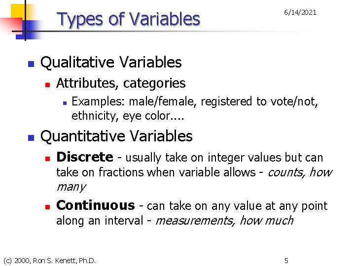
Types of Variables n Qualitative Variables n Attributes, categories n n 6/14/2021 Examples: male/female, registered to vote/not, ethnicity, eye color. . Quantitative Variables n Discrete - usually take on integer values but can take on fractions when variable allows - counts, how many n Continuous - can take on any value at any point along an interval - measurements, how much (c) 2000, Ron S. Kenett, Ph. D. 5
Self Assessment Test 6/14/2021 For each of the following, indicate whether the appropriate variable would be qualitative or quantitative. If the variable is quantitative, indicate whether it would be discrete or continuous. (c) 2000, Ron S. Kenett, Ph. D. 6
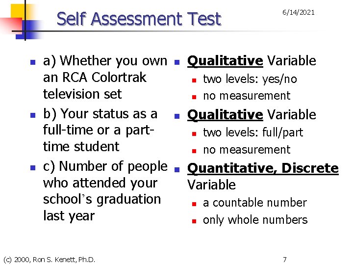
Self Assessment Test n n n a) Whether you own an RCA Colortrak television set b) Your status as a full-time or a parttime student c) Number of people who attended your school’s graduation last year (c) 2000, Ron S. Kenett, Ph. D. n Qualitative Variable n n n two levels: yes/no no measurement Qualitative Variable n n n 6/14/2021 two levels: full/part no measurement Quantitative, Discrete Variable n n a countable number only whole numbers 7
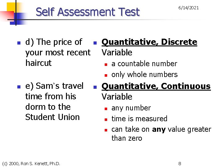
Self Assessment Test n d) The price of your most recent haircut n Quantitative, Discrete Variable n n n e) Sam’s travel time from his dorm to the Student Union n a countable number only whole numbers Quantitative, Continuous Variable n n n (c) 2000, Ron S. Kenett, Ph. D. 6/14/2021 any number time is measured can take on any value greater than zero 8
Self Assessment Test n f) The number of students on campus who belong to a social fraternity or sorority (c) 2000, Ron S. Kenett, Ph. D. n 6/14/2021 Quantitative, Discrete Variable n n a countable number only whole numbers 9
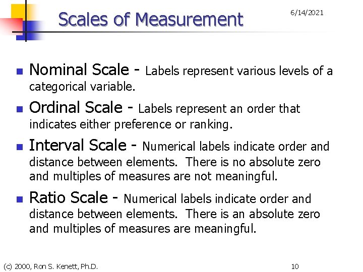
Scales of Measurement n Nominal Scale - 6/14/2021 Labels represent various levels of a categorical variable. n Ordinal Scale - n Interval Scale - n Ratio Scale - Labels represent an order that indicates either preference or ranking. Numerical labels indicate order and distance between elements. There is no absolute zero and multiples of measures are not meaningful. Numerical labels indicate order and distance between elements. There is an absolute zero and multiples of measures are meaningful. (c) 2000, Ron S. Kenett, Ph. D. 10

Self Assessment Test 6/14/2021 Bill scored 1200 on the Scholastic Aptitude Test and entered college as a physics major. As a freshman, he changed to business because he thought it was more interesting. Because he made the dean’s list last semester, his parents gave him $30 to buy a new Casio calculator. Identify at least one piece of information in the: (c) 2000, Ron S. Kenett, Ph. D. 11
Self Assessment Test n a) nominal scale of measurement. (c) 2000, Ron S. Kenett, Ph. D. n 6/14/2021 1. Bill is going to college. 2. Bill will buy a Casio calculator. 3. Bill was a physics major. 4. Bill is a business major. 5. Bill was on the dean’s list. 12
Self Assessment Test n n n b) ordinal scale of measurement c) interval scale of measurement d) ratio scale of measurement (c) 2000, Ron S. Kenett, Ph. D. n n n 6/14/2021 Bill is a freshman. Bill earned a 1200 on the SAT. Bill’s parents gave him $30. 13

Self Assessment Test n n n b) ordinal scale of measurement c) interval scale of measurement d) ratio scale of measurement (c) 2000, Ron S. Kenett, Ph. D. n n n 6/14/2021 Bill is a freshman. Bill earned a 1200 on the SAT. Bill’s parents gave him $30. 14
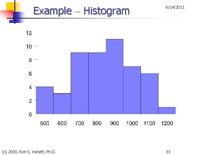
6/14/2021 Histogram A histogram is a way of summarising data that are measured on an interval scale (either discrete or continuous). It is often used in exploratory data analysis to illustrate the major features of the distribution of the data in a convenient form. It divides up the range of possible values in a data set into classes or groups. For each group, a rectangle is constructed with a base length equal to the range of values in that specific group, and an area proportional to the number of observations falling into that group. This means that the rectangles might be drawn of non uniform height. (c) 2000, Ron S. Kenett, Ph. D. 15
Key Terms n Data array n n 6/14/2021 An orderly presentation of data in either ascending or descending numerical order. Frequency Distribution n A table that represents the data in classes and that shows the number of observations in each class. (c) 2000, Ron S. Kenett, Ph. D. 16
Key Terms n 6/14/2021 Frequency Distribution n n Class - The category Frequency - Number in each class Class limits - Boundaries for each class Class interval - Width of each class Class mark - Midpoint of each class (c) 2000, Ron S. Kenett, Ph. D. 17
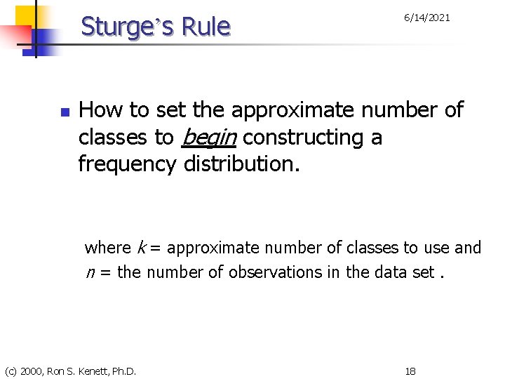
Sturge’s Rule n 6/14/2021 How to set the approximate number of classes to begin constructing a frequency distribution. where k = approximate number of classes to use and n = the number of observations in the data set. (c) 2000, Ron S. Kenett, Ph. D. 18
Frequency Distributions 6/14/2021 1. Number of classes Choose an approximate number of classes for your data. Sturges’ rule can help. 2. Estimate the class interval Divide the approximate number of classes (from Step 1) into the range of your data to find the approximate class interval, where the range is defined as the largest data value minus the smallest data value. 3. Determine the class interval Round the estimate (from Step 2) to a convenient value. (c) 2000, Ron S. Kenett, Ph. D. 19
Frequency Distributions 6/14/2021 4. Lower Class Limit Determine the lower class limit for the first class by selecting a convenient number that is smaller than the lowest data value. 5. Class Limits Determine the other class limits by repeatedly adding the class width (from Step 2) to the prior class limit, starting with the lower class limit (from Step 3). 6. Define the classes Use the sequence of class limits to define the classes. (c) 2000, Ron S. Kenett, Ph. D. 20
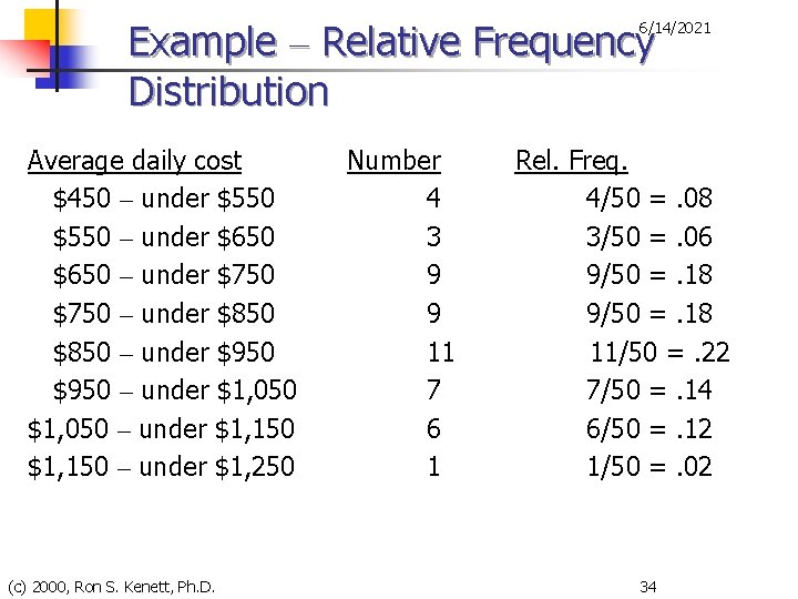
Relative Frequency Distributions 6/14/2021 1. Retain the same classes defined in the frequency distribution. 2. Sum the total number of observations across all classes of the frequency distribution. 3. Divide the frequency for each class by the total number of observations, forming the percentage of data values in each class. (c) 2000, Ron S. Kenett, Ph. D. 21
Cumulative Relative Frequency Distributions 6/14/2021 1. List the number of observations in the lowest class. 2. Add the frequency of the lowest class to the frequency of the second class. Record that cumulative sum for the second class. 3. Continue to add the prior cumulative sum to the frequency for that class, so that the cumulative sum for the final class is the total number of observations in the data set. (c) 2000, Ron S. Kenett, Ph. D. 22
Cumulative Relative Frequency Distributions 6/14/2021 4. Divide the accumulated frequencies for each class by the total number of observations -giving you the percent of all observations that occurred up to an including that class. n An Alternative: Accrue the relative frequencies for each class instead of the raw frequencies. Then you don’t have to divide by the total to get percentages. (c) 2000, Ron S. Kenett, Ph. D. 23
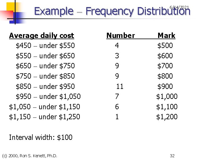
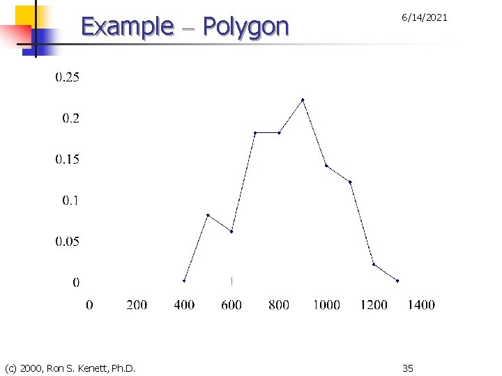
Example n 6/14/2021 The average daily cost to community hospitals for patient stays during 1993 for each of the 50 U. S. states was given in the next table. n n n a) Arrange these into a data array. b) Construct a stem-and-leaf display. *) Approximately how many classes would be appropriate for these data? c & d) Construct a frequency distribution. State interval width and class mark. e) Construct a histogram, a relative frequency distribution, and a cumulative relative frequency distribution. (c) 2000, Ron S. Kenett, Ph. D. 24
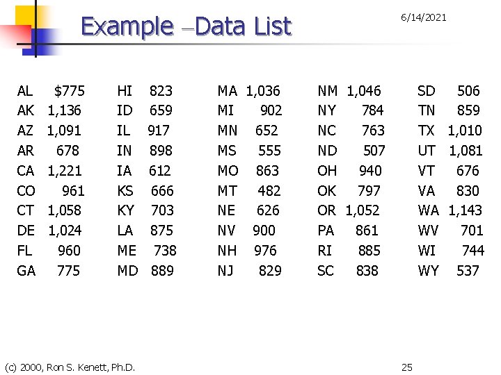
Example –Data List AL AK AZ AR CA CO CT DE FL GA $775 1, 136 1, 091 678 1, 221 961 1, 058 1, 024 960 775 HI ID IL IN IA KS KY LA ME MD (c) 2000, Ron S. Kenett, Ph. D. 823 659 917 898 612 666 703 875 738 889 MA 1, 036 MI 902 MN 652 MS 555 MO 863 MT 482 NE 626 NV 900 NH 976 NJ 829 6/14/2021 NM 1, 046 NY 784 NC 763 ND 507 OH 940 OK 797 OR 1, 052 PA 861 RI 885 SC 838 SD 506 TN 859 TX 1, 010 UT 1, 081 VT 676 VA 830 WA 1, 143 WV 701 WI 744 WY 537 25
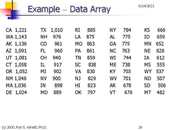
Example – Data Array CA 1, 221 WA 1, 143 AK 1, 136 AZ 1, 091 UT 1, 081 CT 1, 058 OR 1, 052 NM 1, 046 MA 1, 036 DE 1, 024 TX 1, 010 NH 976 CO 961 FL 960 CH 940 IL 917 MI 902 NV 900 IN 898 MD 889 (c) 2000, Ron S. Kenett, Ph. D. RI LA MO PA TN SC VA NJ HI OK 885 875 863 861 859 838 830 829 823 797 NY AL GA NC WI ME KY WV AR VT 6/14/2021 784 775 763 744 738 703 701 678 676 KS 666 ID 659 MN 652 NE 626 IA 612 MS 555 WY 537 ND 507 SD 506 MT 482 26
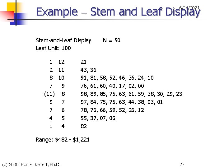
Example – Stem and Leaf Display 6/14/2021 Stem-and-Leaf Display Leaf Unit: 100 1 12 2 11 8 10 7 9 (11) 8 9 7 7 6 4 5 1 4 21 43, 91, 76, 98, 97, 78, 55, 82 36 81, 61, 89, 84, 76, 37, N = 50 58, 60, 85, 75, 66, 07, 52, 40, 75, 59, 06 46, 17, 63, 52, 36, 02, 61, 44, 26, 24, 10 00 59, 38, 30, 29, 23 38, 03, 01 12 Range: $482 - $1, 221 (c) 2000, Ron S. Kenett, Ph. D. 27
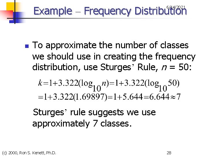
Example – Frequency Distribution 6/14/2021 n To approximate the number of classes we should use in creating the frequency distribution, use Sturges’ Rule, n = 50: Sturges’ rule suggests we use approximately 7 classes. (c) 2000, Ron S. Kenett, Ph. D. 28
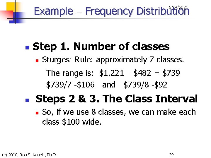
Example – Frequency Distribution 6/14/2021 n Step 1. Number of classes n Sturges’ Rule: approximately 7 classes. The range is: $1, 221 – $482 = $739/7 $106 and $739/8 $92 n Steps 2 & 3. The Class Interval n So, if we use 8 classes, we can make each class $100 wide. (c) 2000, Ron S. Kenett, Ph. D. 29

Example – Frequency Distribution 6/14/2021 n Step 1. Number of classes n Sturges’ Rule: approximately 7 classes. The range is: $1, 221 – $482 = $739/7 $106 and $739/8 $92 n Steps 2 & 3. The Class Interval n So, if we use 8 classes, we can make each class $100 wide. (c) 2000, Ron S. Kenett, Ph. D. 30
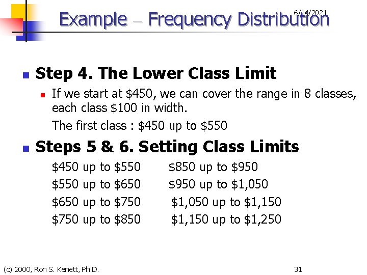
Example – Frequency Distribution 6/14/2021 n Step 4. The Lower Class Limit n n If we start at $450, we can cover the range in 8 classes, each class $100 in width. The first class : $450 up to $550 Steps 5 & 6. Setting Class Limits $450 $550 $650 $750 up up (c) 2000, Ron S. Kenett, Ph. D. to to $550 $650 $750 $850 up to $950 up to $1, 050 up to $1, 150 up to $1, 250 31
Example – Frequency Distribution 6/14/2021 Average daily cost $450 – under $550 – under $650 – under $750 – under $850 – under $950 – under $1, 050 – under $1, 150 – under $1, 250 Number 4 3 9 9 11 7 6 1 Mark $500 $600 $700 $800 $900 $1, 000 $1, 100 $1, 200 Interval width: $100 (c) 2000, Ron S. Kenett, Ph. D. 32
Example – Histogram (c) 2000, Ron S. Kenett, Ph. D. 6/14/2021 33
Example – Relative Frequency Distribution 6/14/2021 Average daily cost $450 – under $550 – under $650 – under $750 – under $850 – under $950 – under $1, 050 – under $1, 150 – under $1, 250 (c) 2000, Ron S. Kenett, Ph. D. Number 4 3 9 9 11 7 6 1 Rel. Freq. 4/50 =. 08 3/50 =. 06 9/50 =. 18 11/50 =. 22 7/50 =. 14 6/50 =. 12 1/50 =. 02 34
Example – Polygon (c) 2000, Ron S. Kenett, Ph. D. 6/14/2021 35
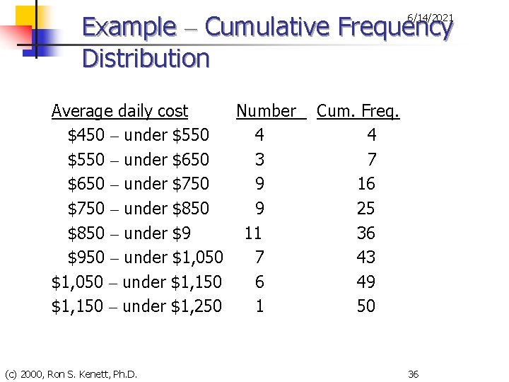
Example – Cumulative Frequency Distribution 6/14/2021 Average daily cost Number $450 – under $550 4 $550 – under $650 3 $650 – under $750 9 $750 – under $850 9 $850 – under $9 11 $950 – under $1, 050 7 $1, 050 – under $1, 150 6 $1, 150 – under $1, 250 1 (c) 2000, Ron S. Kenett, Ph. D. Cum. Freq. 4 7 16 25 36 43 49 50 36
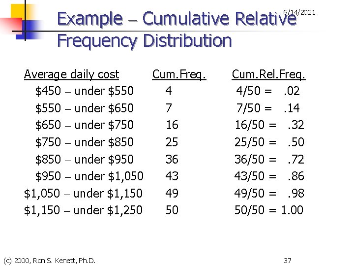
Example – Cumulative Relative Frequency Distribution 6/14/2021 Average daily cost Cum. Freq. $450 – under $550 4 $550 – under $650 7 $650 – under $750 16 $750 – under $850 25 $850 – under $950 36 $950 – under $1, 050 43 $1, 050 – under $1, 150 49 $1, 150 – under $1, 250 50 (c) 2000, Ron S. Kenett, Ph. D. Cum. Rel. Freq. 4/50 =. 02 7/50 =. 14 16/50 =. 32 25/50 =. 50 36/50 =. 72 43/50 =. 86 49/50 =. 98 50/50 = 1. 00 37
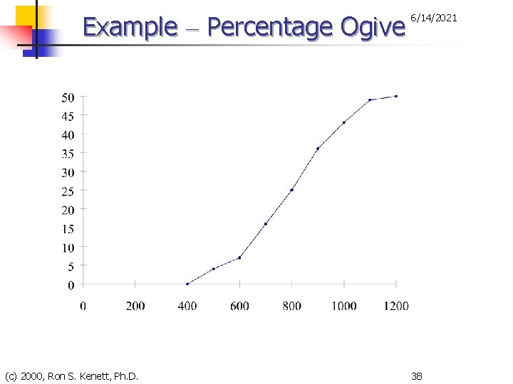
Example – Percentage Ogive (c) 2000, Ron S. Kenett, Ph. D. 6/14/2021 38
6/14/2021 (c) 2000, Ron S. Kenett, Ph. D. 39
Key Terms n Measures of Central Tendency, The Center n Mean n n (c) 2000, Ron S. Kenett, Ph. D. 6/14/2021 µ, population; , sample Weighted Mean Median Mode 40
Key Terms n Measures of Dispersion, The Spread n n n n (c) 2000, Ron S. Kenett, Ph. D. 6/14/2021 Range Mean absolute deviation Variance Standard deviation Interquartile range Interquartile deviation Coefficient of variation 41
Key Terms n Measures of Relative Position 6/14/2021 n Quantiles n n n (c) 2000, Ron S. Kenett, Ph. D. Quartiles Deciles Percentiles Residuals Standardized values 42
The Mean n 6/14/2021 Mean n Arithmetic average = (sum all values)/# of values n n Population: µ = (Sxi)/N Sample: = (Sxi)/n Problem: Calculate the average number of truck shipments from the United States to five Canadian cities for the following data given in thousands of bags: Montreal, 64. 0; Ottawa, 15. 0; Toronto, 285. 0; Vancouver, 228. 0; Winnipeg, 45. 0 (Ans: 127. 4) (c) 2000, Ron S. Kenett, Ph. D. 43
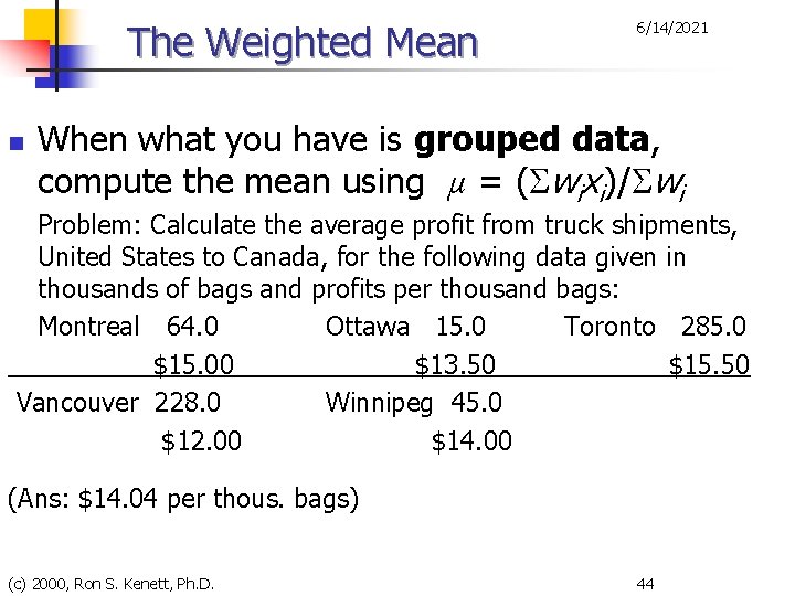
The Weighted Mean n 6/14/2021 When what you have is grouped data, compute the mean using µ = (Swixi)/Swi Problem: Calculate the average profit from truck shipments, United States to Canada, for the following data given in thousands of bags and profits per thousand bags: Montreal 64. 0 Ottawa 15. 0 Toronto 285. 0 $15. 00 $13. 50 $15. 50 Vancouver 228. 0 Winnipeg 45. 0 $12. 00 $14. 00 (Ans: $14. 04 per thous. bags) (c) 2000, Ron S. Kenett, Ph. D. 44
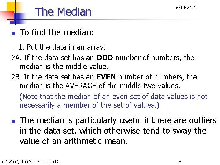
The Median n 6/14/2021 To find the median: 1. Put the data in an array. 2 A. If the data set has an ODD number of numbers, the median is the middle value. 2 B. If the data set has an EVEN number of numbers, the median is the AVERAGE of the middle two values. (Note that the median of an even set of data values is not necessarily a member of the set of values. ) n The median is particularly useful if there are outliers in the data set, which otherwise tend to sway the value of an arithmetic mean. (c) 2000, Ron S. Kenett, Ph. D. 45
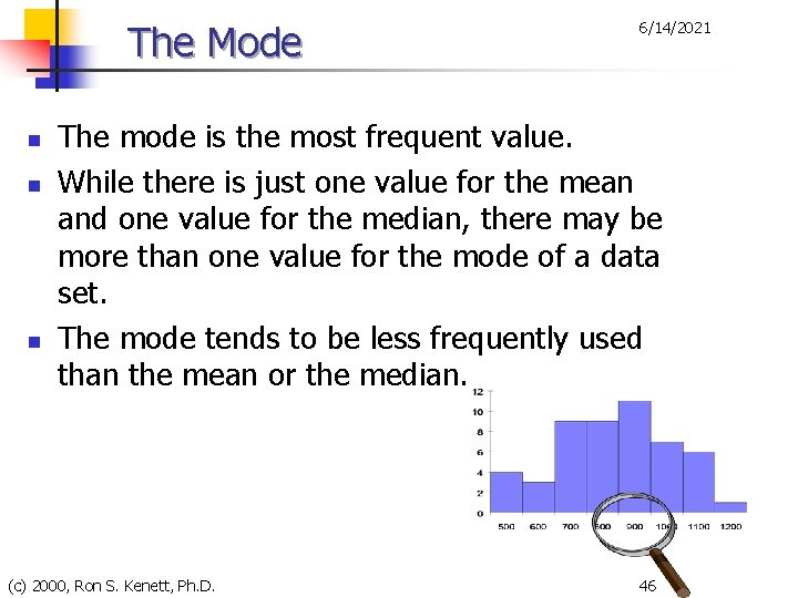
The Mode n n n 6/14/2021 The mode is the most frequent value. While there is just one value for the mean and one value for the median, there may be more than one value for the mode of a data set. The mode tends to be less frequently used than the mean or the median. (c) 2000, Ron S. Kenett, Ph. D. 46
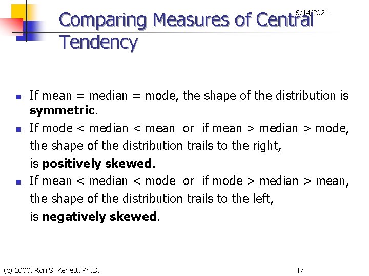
Comparing Measures of Central Tendency 6/14/2021 n n n If mean = median = mode, the shape of the distribution is symmetric. If mode < median < mean or if mean > median > mode, the shape of the distribution trails to the right, is positively skewed. If mean < median < mode or if mode > median > mean, the shape of the distribution trails to the left, is negatively skewed. (c) 2000, Ron S. Kenett, Ph. D. 47
The Range n n n 6/14/2021 The range is the distance between the smallest and the largest data value in the set. Range = largest value – smallest value Sometimes range is reported as an interval, anchored between the smallest and largest data value, rather than the actual width of that interval. (c) 2000, Ron S. Kenett, Ph. D. 48
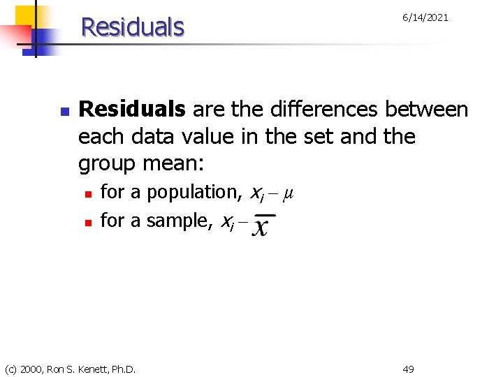
Residuals n 6/14/2021 Residuals are the differences between each data value in the set and the group mean: n n for a population, xi – µ for a sample, xi – (c) 2000, Ron S. Kenett, Ph. D. 49
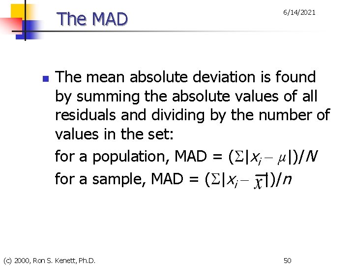
The MAD n 6/14/2021 The mean absolute deviation is found by summing the absolute values of all residuals and dividing by the number of values in the set: for a population, MAD = (S|xi – µ|)/N for a sample, MAD = (S|xi – |)/n (c) 2000, Ron S. Kenett, Ph. D. 50
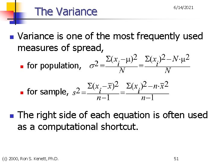
The Variance n n 6/14/2021 Variance is one of the most frequently used measures of spread, n for population, n for sample, The right side of each equation is often used as a computational shortcut. (c) 2000, Ron S. Kenett, Ph. D. 51
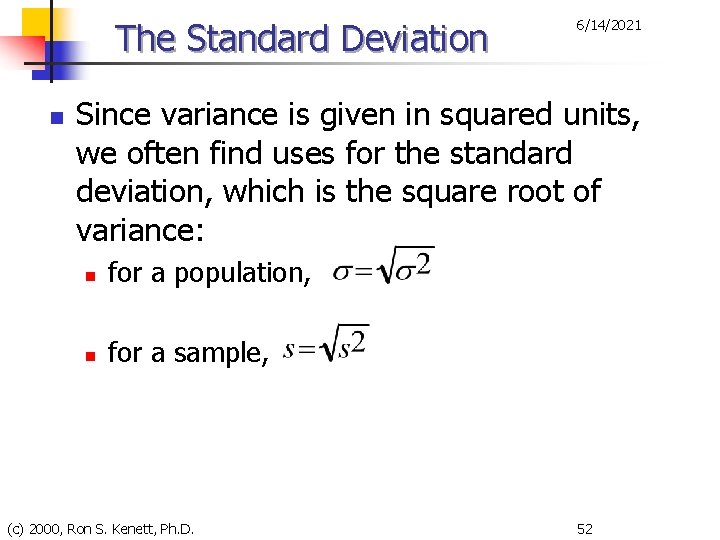
The Standard Deviation n 6/14/2021 Since variance is given in squared units, we often find uses for the standard deviation, which is the square root of variance: n for a population, n for a sample, (c) 2000, Ron S. Kenett, Ph. D. 52
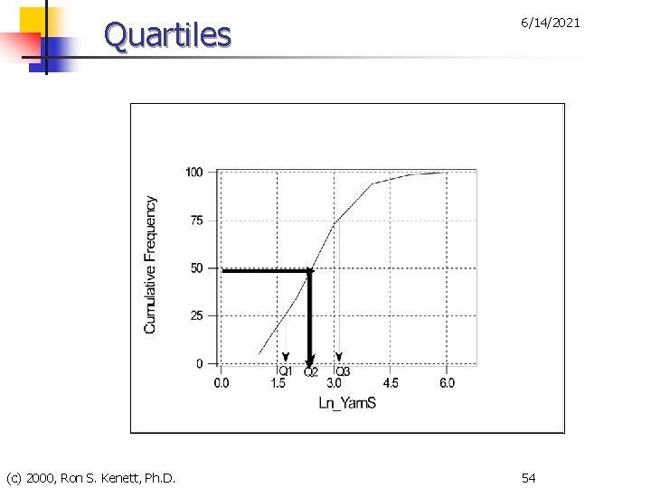
Quartiles n n n 6/14/2021 One of the most frequently used quantiles is the quartile. Quartiles divide the values of a data set into four subsets of equal size, each comprising 25% of the observations. To find the first, second, and third quartiles: n n 1. 2. 3. 4. Arrange the N data values into an array. First quartile, Q 1 = data value at position (N + 1)/4 Second quartile, Q 2 = data value at position 2(N + 1)/4 Third quartile, Q 3 = data value at position 3(N + 1)/4 (c) 2000, Ron S. Kenett, Ph. D. 53
Quartiles (c) 2000, Ron S. Kenett, Ph. D. 6/14/2021 54
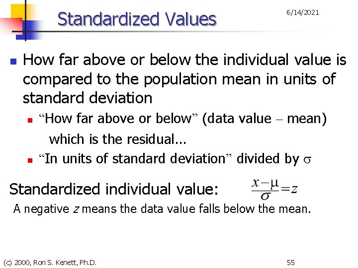
Standardized Values n 6/14/2021 How far above or below the individual value is compared to the population mean in units of standard deviation n n “How far above or below” (data value – mean) which is the residual. . . “In units of standard deviation” divided by s Standardized individual value: A negative z means the data value falls below the mean. (c) 2000, Ron S. Kenett, Ph. D. 55
- Slides: 55