6 The Circular Functions and Their Graphs Sections


- Slides: 72

6 The Circular Functions and Their Graphs Sections 6. 1– 6. 4 © 2008 Pearson Addison-Wesley. All rights reserved

6 The Circular Functions and Their Graphs 6. 1 Radian Measure 6. 2 The Unit Circle and Circular Functions 6. 3 Graphs of the Sine and Cosine Functions 6. 4 Translations of the Graphs of the Sine and Cosine Functions 2 Copyright © 2008 Pearson Addison-Wesley. All rights reserved.

6. 1 Radian Measure ▪ Converting Between Degrees and Radians ▪ Arc Length of a Circle ▪ Area of a Sector of a Circle 3 Copyright © 2008 Pearson Addison-Wesley. All rights reserved.

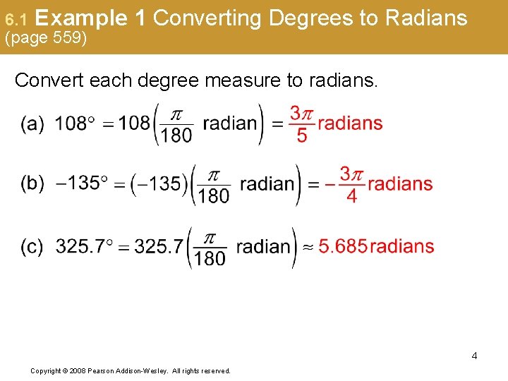
6. 1 Example (page 559) 1 Converting Degrees to Radians Convert each degree measure to radians. 4 Copyright © 2008 Pearson Addison-Wesley. All rights reserved.

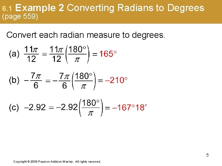
6. 1 Example (page 559) 2 Converting Radians to Degrees Convert each radian measure to degrees. 5 Copyright © 2008 Pearson Addison-Wesley. All rights reserved.

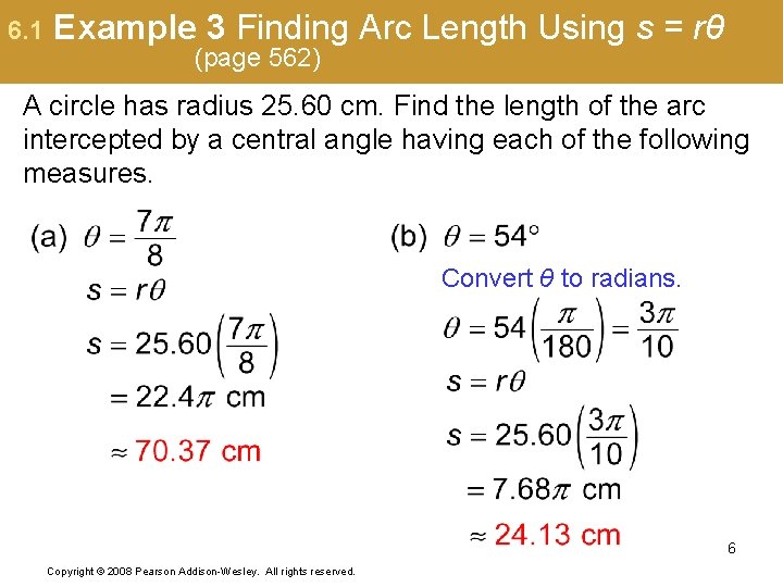
6. 1 Example 3 Finding Arc Length Using s = rθ (page 562) A circle has radius 25. 60 cm. Find the length of the arc intercepted by a central angle having each of the following measures. Convert θ to radians. 6 Copyright © 2008 Pearson Addison-Wesley. All rights reserved.

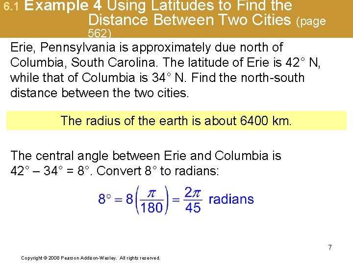
6. 1 Example 4 Using Latitudes to Find the Distance Between Two Cities (page 562) Erie, Pennsylvania is approximately due north of Columbia, South Carolina. The latitude of Erie is 42° N, while that of Columbia is 34° N. Find the north-south distance between the two cities. The radius of the earth is about 6400 km. The central angle between Erie and Columbia is 42° – 34° = 8°. Convert 8° to radians: 7 Copyright © 2008 Pearson Addison-Wesley. All rights reserved.

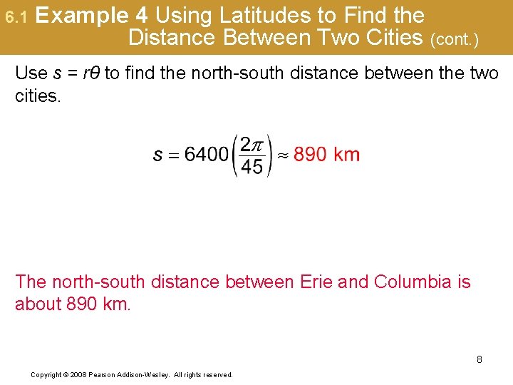
6. 1 Example 4 Using Latitudes to Find the Distance Between Two Cities (cont. ) Use s = rθ to find the north-south distance between the two cities. The north-south distance between Erie and Columbia is about 890 km. 8 Copyright © 2008 Pearson Addison-Wesley. All rights reserved.

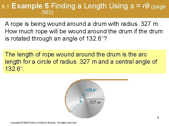
6. 1 Example 5 Finding a Length Using s = rθ (page 563) A rope is being wound around a drum with radius. 327 m. How much rope will be wound around the drum if the drum is rotated through an angle of 132. 6°? The length of rope wound around the drum is the arc length for a circle of radius. 327 m and a central angle of 132. 6°. 9 Copyright © 2008 Pearson Addison-Wesley. All rights reserved.

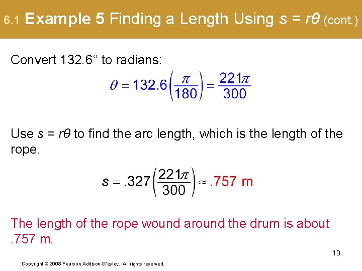
6. 1 Example 5 Finding a Length Using s = rθ (cont. ) Convert 132. 6° to radians: Use s = rθ to find the arc length, which is the length of the rope. The length of the rope wound around the drum is about. 757 m. 10 Copyright © 2008 Pearson Addison-Wesley. All rights reserved.

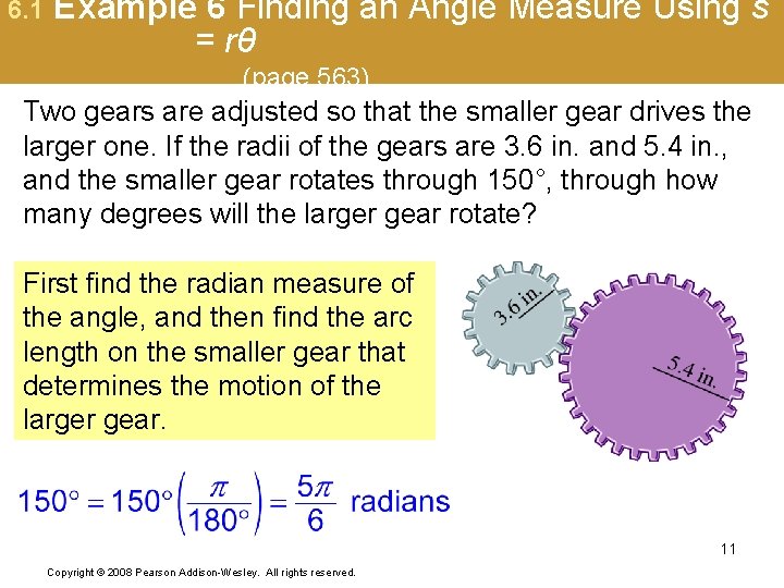
6. 1 Example 6 Finding an Angle Measure Using s = rθ (page 563) Two gears are adjusted so that the smaller gear drives the larger one. If the radii of the gears are 3. 6 in. and 5. 4 in. , and the smaller gear rotates through 150°, through how many degrees will the larger gear rotate? First find the radian measure of the angle, and then find the arc length on the smaller gear that determines the motion of the larger gear. 11 Copyright © 2008 Pearson Addison-Wesley. All rights reserved.

6. 1 Example 6 Finding an Angle Measure Using s = rθ (cont. ) The arc length on the smaller gear is An arc with length 3π cm on the larger gear corresponds to an angle measure θ radians, where The larger gear will rotate through 100°. Copyright © 2008 Pearson Addison-Wesley. All rights reserved. 12

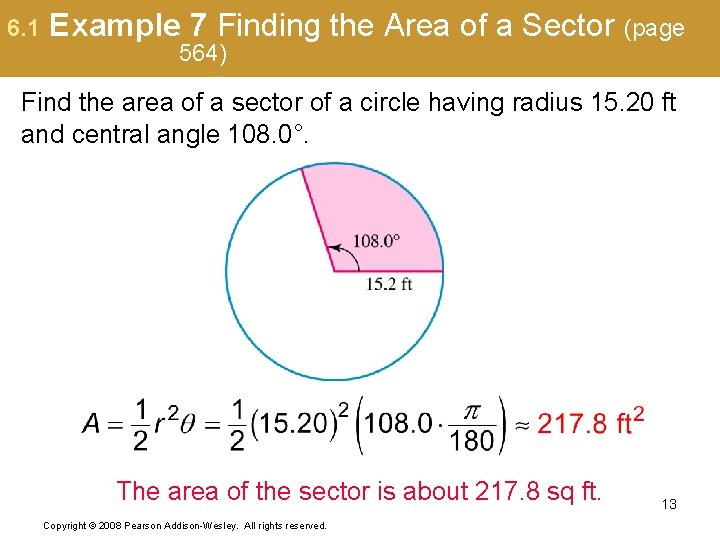
6. 1 Example 7 Finding the Area of a Sector (page 564) Find the area of a sector of a circle having radius 15. 20 ft and central angle 108. 0°. The area of the sector is about 217. 8 sq ft. Copyright © 2008 Pearson Addison-Wesley. All rights reserved. 13

6. 2 The Unit Circle and Circular Functions ▪ Finding Values of Circular Functions ▪ Determining a Number with a Given Circular Function Value ▪ Linear and Angular Speed 14 Copyright © 2008 Pearson Addison-Wesley. All rights reserved.

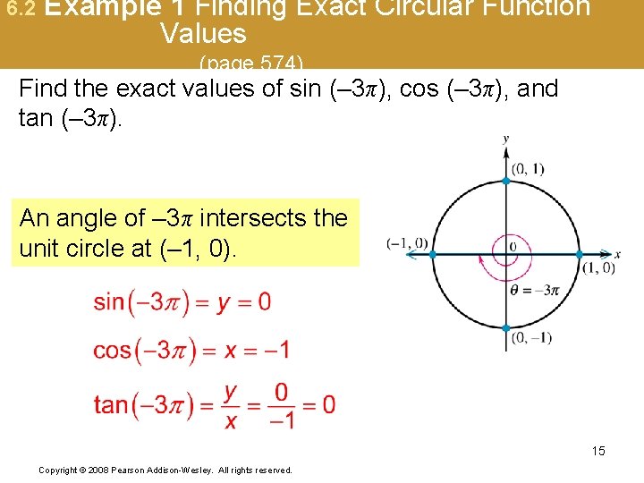
6. 2 Example 1 Finding Exact Circular Function Values (page 574) Find the exact values of sin (– 3π), cos (– 3π), and tan (– 3π). An angle of – 3π intersects the unit circle at (– 1, 0). 15 Copyright © 2008 Pearson Addison-Wesley. All rights reserved.

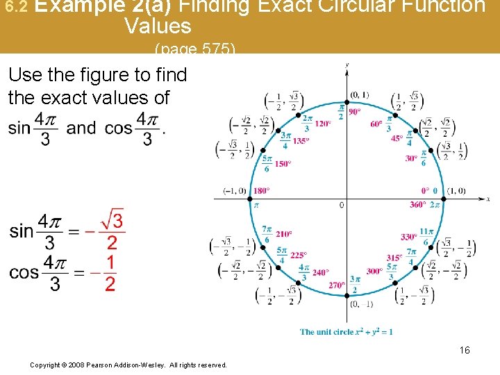
6. 2 Example 2(a) Finding Exact Circular Function Values (page 575) Use the figure to find the exact values of 16 Copyright © 2008 Pearson Addison-Wesley. All rights reserved.

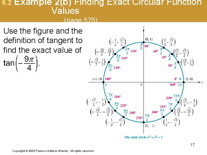
6. 2 Example 2(b) Finding Exact Circular Function Values (page 575) Use the figure and the definition of tangent to find the exact value of 17 Copyright © 2008 Pearson Addison-Wesley. All rights reserved.

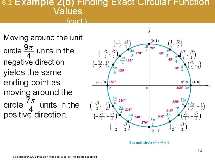
6. 2 Example 2(b) Finding Exact Circular Function Values (cont. ) Moving around the unit circle units in the negative direction yields the same ending point as moving around the circle units in the positive direction. 18 Copyright © 2008 Pearson Addison-Wesley. All rights reserved.

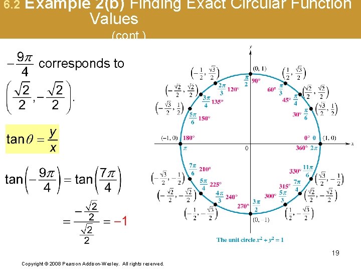
6. 2 Example 2(b) Finding Exact Circular Function Values (cont. ) corresponds to 19 Copyright © 2008 Pearson Addison-Wesley. All rights reserved.

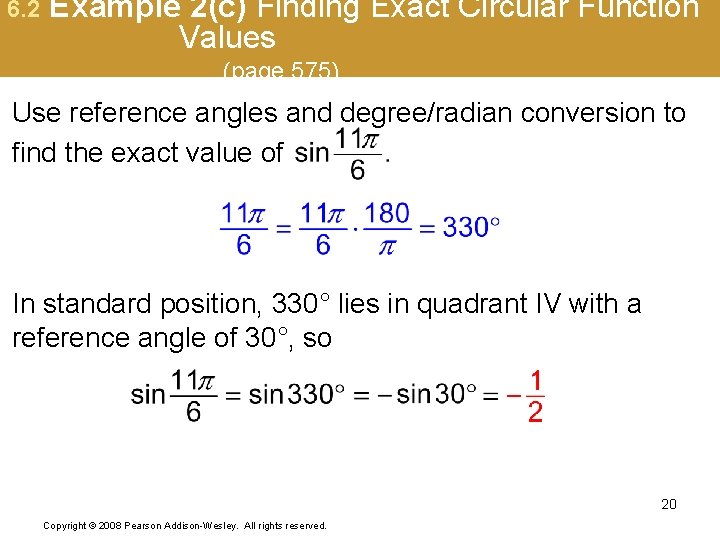
6. 2 Example 2(c) Finding Exact Circular Function Values (page 575) Use reference angles and degree/radian conversion to find the exact value of In standard position, 330° lies in quadrant IV with a reference angle of 30°, so 20 Copyright © 2008 Pearson Addison-Wesley. All rights reserved.

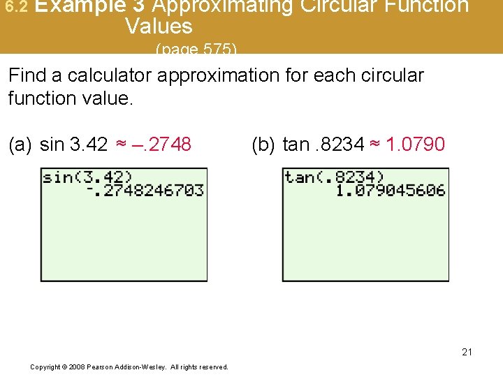
6. 2 Example 3 Approximating Circular Function Values (page 575) Find a calculator approximation for each circular function value. (a) sin 3. 42 ≈ –. 2748 (b) tan. 8234 ≈ 1. 0790 21 Copyright © 2008 Pearson Addison-Wesley. All rights reserved.

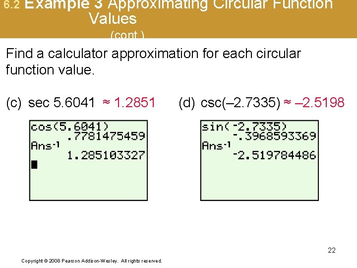
6. 2 Example 3 Approximating Circular Function Values (cont. ) Find a calculator approximation for each circular function value. (c) sec 5. 6041 ≈ 1. 2851 (d) csc(– 2. 7335) ≈ – 2. 5198 22 Copyright © 2008 Pearson Addison-Wesley. All rights reserved.

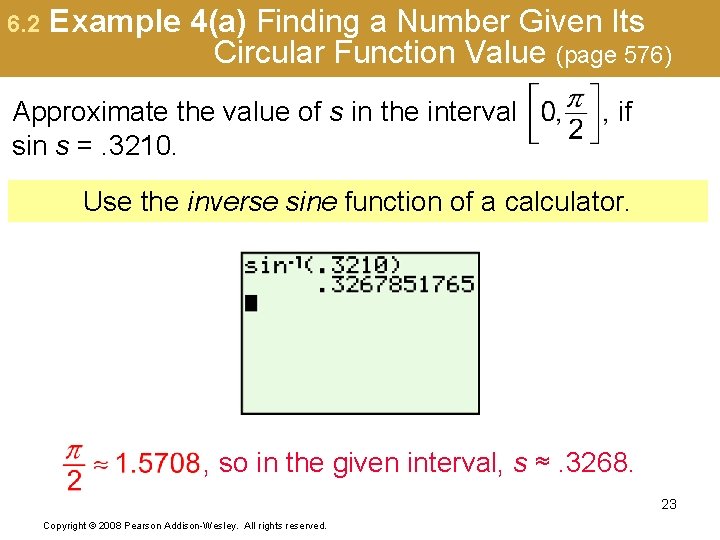
6. 2 Example 4(a) Finding a Number Given Its Circular Function Value (page 576) Approximate the value of s in the interval sin s =. 3210. if Use the inverse sine function of a calculator. , so in the given interval, s ≈. 3268. 23 Copyright © 2008 Pearson Addison-Wesley. All rights reserved.

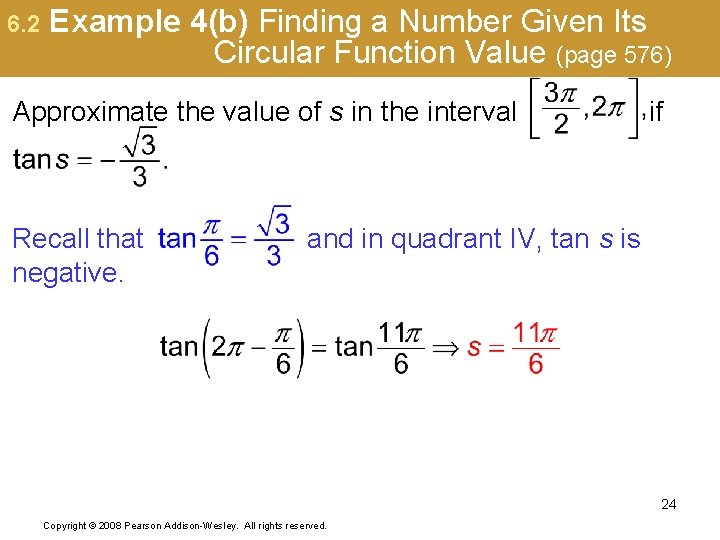
6. 2 Example 4(b) Finding a Number Given Its Circular Function Value (page 576) Approximate the value of s in the interval Recall that negative. if and in quadrant IV, tan s is 24 Copyright © 2008 Pearson Addison-Wesley. All rights reserved.

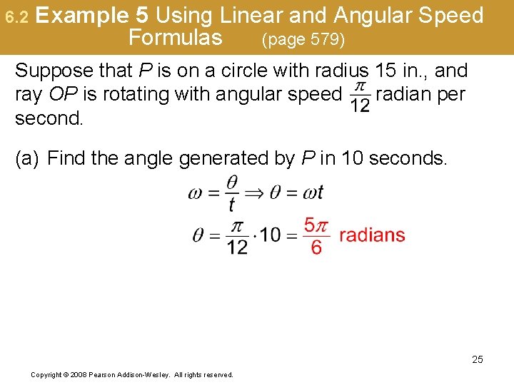
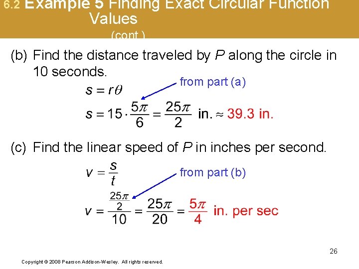
6. 2 Example 5 Using Linear and Angular Speed Formulas (page 579) Suppose that P is on a circle with radius 15 in. , and ray OP is rotating with angular speed radian per second. (a) Find the angle generated by P in 10 seconds. 25 Copyright © 2008 Pearson Addison-Wesley. All rights reserved.

6. 2 Example 5 Finding Exact Circular Function Values (cont. ) (b) Find the distance traveled by P along the circle in 10 seconds. from part (a) (c) Find the linear speed of P in inches per second. from part (b) 26 Copyright © 2008 Pearson Addison-Wesley. All rights reserved.

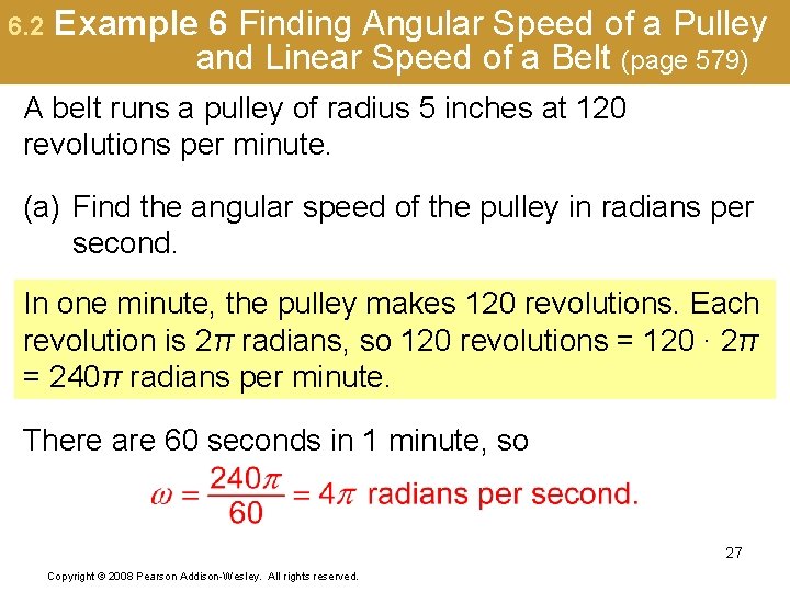
6. 2 Example 6 Finding Angular Speed of a Pulley and Linear Speed of a Belt (page 579) A belt runs a pulley of radius 5 inches at 120 revolutions per minute. (a) Find the angular speed of the pulley in radians per second. In one minute, the pulley makes 120 revolutions. Each revolution is 2π radians, so 120 revolutions = 120 ∙ 2π = 240π radians per minute. There are 60 seconds in 1 minute, so 27 Copyright © 2008 Pearson Addison-Wesley. All rights reserved.

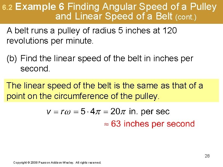
6. 2 Example 6 Finding Angular Speed of a Pulley and Linear Speed of a Belt (cont. ) A belt runs a pulley of radius 5 inches at 120 revolutions per minute. (b) Find the linear speed of the belt in inches per second. The linear speed of the belt is the same as that of a point on the circumference of the pulley. 28 Copyright © 2008 Pearson Addison-Wesley. All rights reserved.

6. 3 Graphs of the Sine and Cosine Functions Periodic Functions ▪ Graph of the Sine Function▪ Graph of the Cosine Function ▪ Graphing Techniques, Amplitude, and Period ▪ Using a Trigonometric Model 29 Copyright © 2008 Pearson Addison-Wesley. All rights reserved.

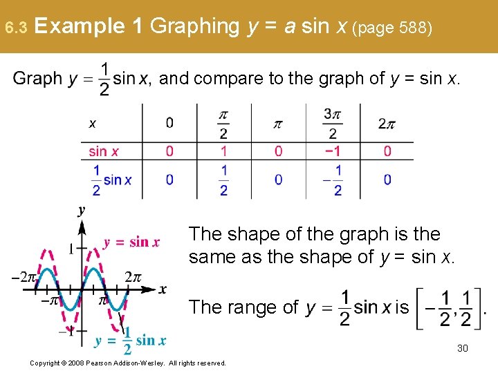
6. 3 Example 1 Graphing y = a sin x (page 588) and compare to the graph of y = sin x. The shape of the graph is the same as the shape of y = sin x. The range of is 30 Copyright © 2008 Pearson Addison-Wesley. All rights reserved.

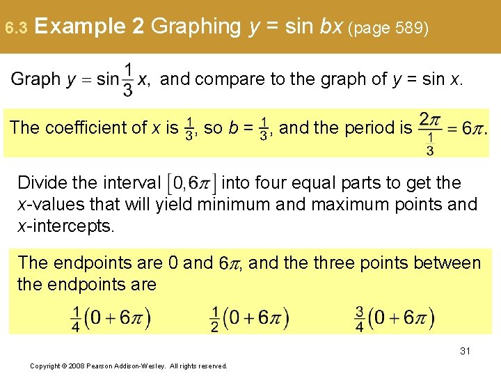
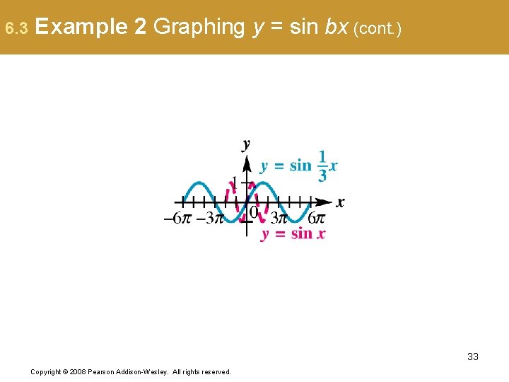
6. 3 Example 2 Graphing y = sin bx (page 589) and compare to the graph of y = sin x. The coefficient of x is , so b = , and the period is Divide the interval into four equal parts to get the x-values that will yield minimum and maximum points and x-intercepts. The endpoints are 0 and the endpoints are , and the three points between 31 Copyright © 2008 Pearson Addison-Wesley. All rights reserved.

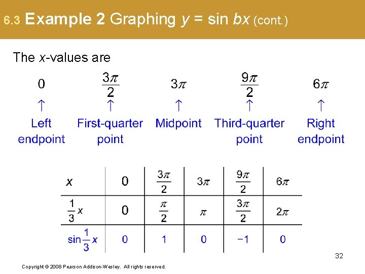
6. 3 Example 2 Graphing y = sin bx (cont. ) The x-values are 32 Copyright © 2008 Pearson Addison-Wesley. All rights reserved.

6. 3 Example 2 Graphing y = sin bx (cont. ) 33 Copyright © 2008 Pearson Addison-Wesley. All rights reserved.

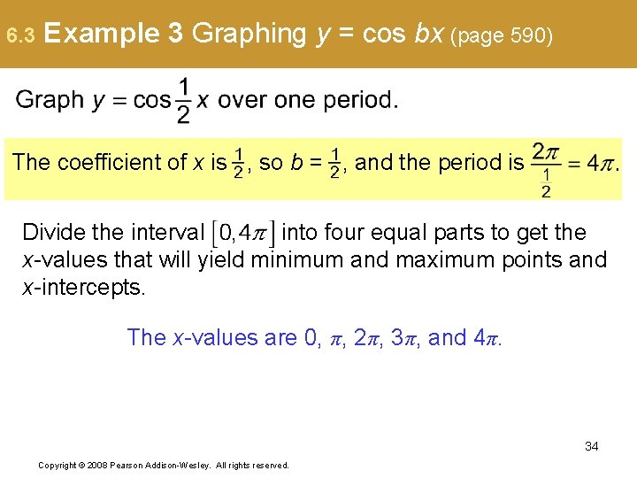
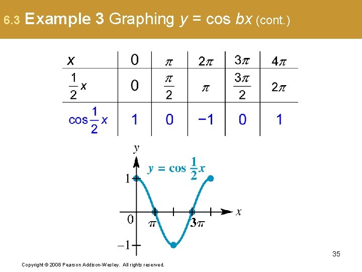
6. 3 Example 3 Graphing y = cos bx (page 590) The coefficient of x is , so b = , and the period is Divide the interval into four equal parts to get the x-values that will yield minimum and maximum points and x-intercepts. The x-values are 0, π, 2π, 3π, and 4π. 34 Copyright © 2008 Pearson Addison-Wesley. All rights reserved.

6. 3 Example 3 Graphing y = cos bx (cont. ) 35 Copyright © 2008 Pearson Addison-Wesley. All rights reserved.

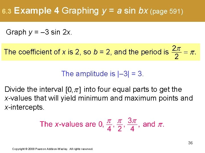
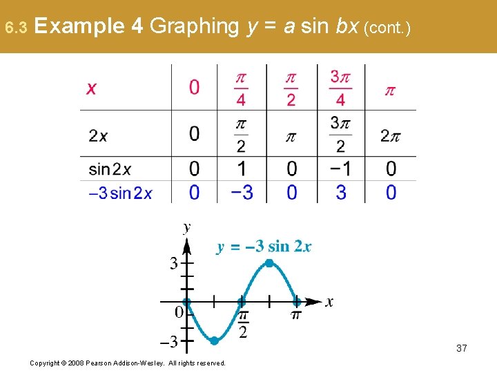
6. 3 Example 4 Graphing y = a sin bx (page 591) Graph y = – 3 sin 2 x. The coefficient of x is 2, so b = 2, and the period is The amplitude is |– 3| = 3. Divide the interval into four equal parts to get the x-values that will yield minimum and maximum points and x-intercepts. 36 Copyright © 2008 Pearson Addison-Wesley. All rights reserved.

6. 3 Example 4 Graphing y = a sin bx (cont. ) 37 Copyright © 2008 Pearson Addison-Wesley. All rights reserved.

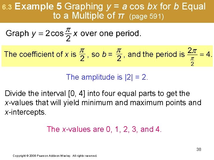
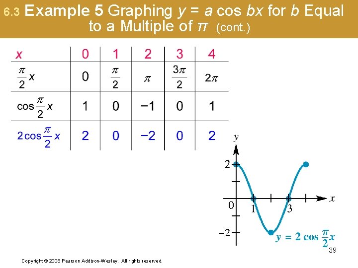
6. 3 Example 5 Graphing y = a cos bx for b Equal to a Multiple of π (page 591) The coefficient of x is , so b = , and the period is The amplitude is |2| = 2. Divide the interval [0, 4] into four equal parts to get the x-values that will yield minimum and maximum points and x-intercepts. The x-values are 0, 1, 2, 3, and 4. 38 Copyright © 2008 Pearson Addison-Wesley. All rights reserved.

6. 3 Example 5 Graphing y = a cos bx for b Equal to a Multiple of π (cont. ) 39 Copyright © 2008 Pearson Addison-Wesley. All rights reserved.

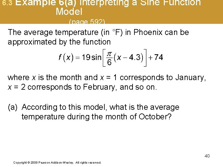
6. 3 Example 6(a) Interpreting a Sine Function Model (page 592) The average temperature (in °F) in Phoenix can be approximated by the function where x is the month and x = 1 corresponds to January, x = 2 corresponds to February, and so on. (a) According to this model, what is the average temperature during the month of October? 40 Copyright © 2008 Pearson Addison-Wesley. All rights reserved.

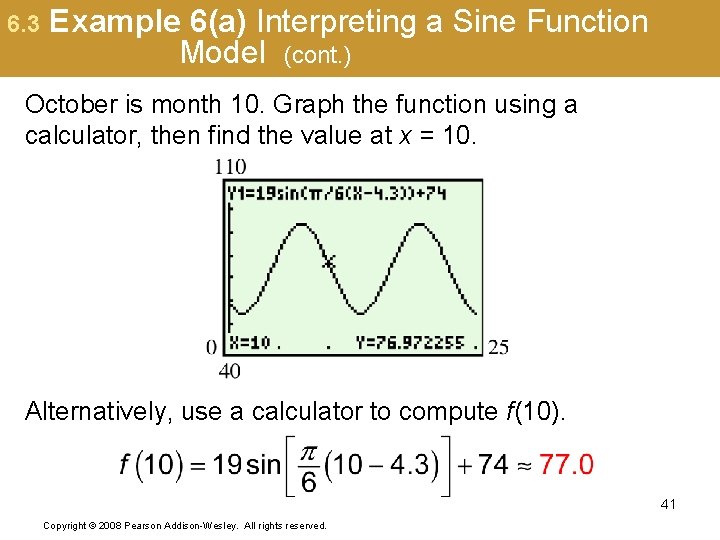
6. 3 Example 6(a) Interpreting a Sine Function Model (cont. ) October is month 10. Graph the function using a calculator, then find the value at x = 10. Alternatively, use a calculator to compute f(10). 41 Copyright © 2008 Pearson Addison-Wesley. All rights reserved.

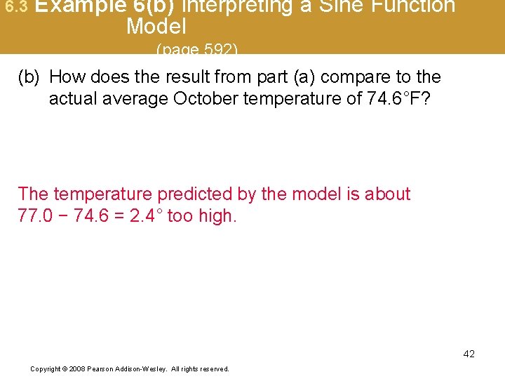
6. 3 Example 6(b) Interpreting a Sine Function Model (page 592) (b) How does the result from part (a) compare to the actual average October temperature of 74. 6°F? The temperature predicted by the model is about 77. 0 − 74. 6 = 2. 4° too high. 42 Copyright © 2008 Pearson Addison-Wesley. All rights reserved.

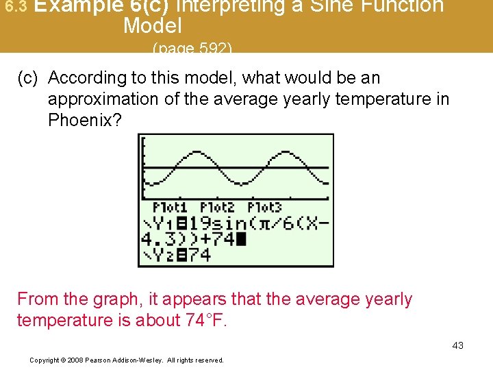
6. 3 Example 6(c) Interpreting a Sine Function Model (page 592) (c) According to this model, what would be an approximation of the average yearly temperature in Phoenix? From the graph, it appears that the average yearly temperature is about 74°F. 43 Copyright © 2008 Pearson Addison-Wesley. All rights reserved.

6. 4 Translations of the Graphs of the Sine and Cosine Functions Horizontal Translations ▪ Vertical Translations ▪ Combinations of Translations ▪ Determining a Trigonometric Model Using Curve Fitting 44 Copyright © 2008 Pearson Addison-Wesley. All rights reserved.

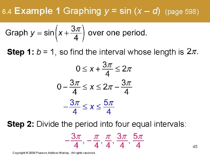
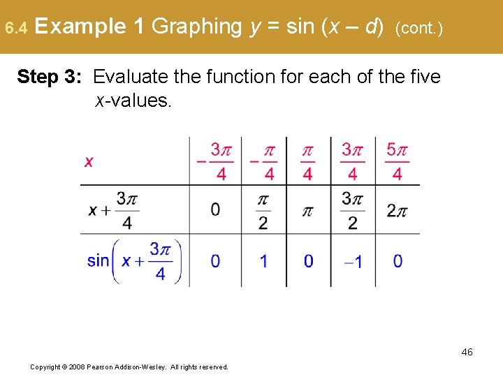
6. 4 Example 1 Graphing y = sin (x – d) (page 598) Step 1: b = 1, so find the interval whose length is Step 2: Divide the period into four equal intervals: 45 Copyright © 2008 Pearson Addison-Wesley. All rights reserved.

6. 4 Example 1 Graphing y = sin (x – d) (cont. ) Step 3: Evaluate the function for each of the five x-values. 46 Copyright © 2008 Pearson Addison-Wesley. All rights reserved.

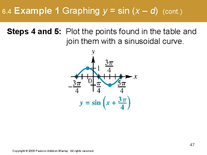
6. 4 Example 1 Graphing y = sin (x – d) (cont. ) Steps 4 and 5: Plot the points found in the table and join them with a sinusoidal curve. 47 Copyright © 2008 Pearson Addison-Wesley. All rights reserved.

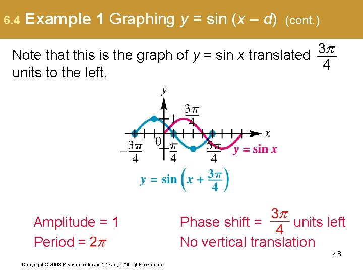
6. 4 Example 1 Graphing y = sin (x – d) (cont. ) Note that this is the graph of y = sin x translated units to the left. Amplitude = 1 Period = Phase shift = units left No vertical translation 48 Copyright © 2008 Pearson Addison-Wesley. All rights reserved.

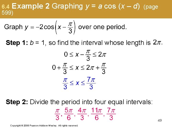
6. 4 Example 599) 2 Graphing y = a cos (x – d) (page Step 1: b = 1, so find the interval whose length is Step 2: Divide the period into four equal intervals: 49 Copyright © 2008 Pearson Addison-Wesley. All rights reserved.

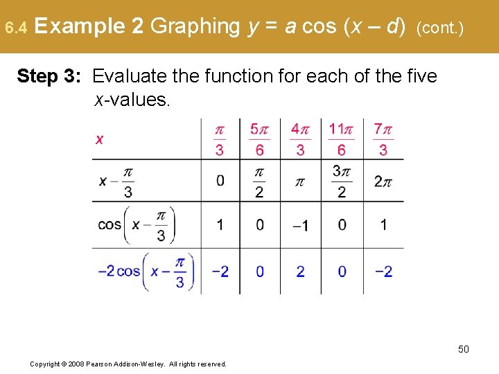
6. 4 Example 2 Graphing y = a cos (x – d) (cont. ) Step 3: Evaluate the function for each of the five x-values. 50 Copyright © 2008 Pearson Addison-Wesley. All rights reserved.

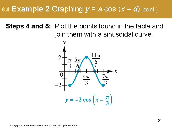
6. 4 Example 2 Graphing y = a cos (x – d) (cont. ) Steps 4 and 5: Plot the points found in the table and join them with a sinusoidal curve. 51 Copyright © 2008 Pearson Addison-Wesley. All rights reserved.

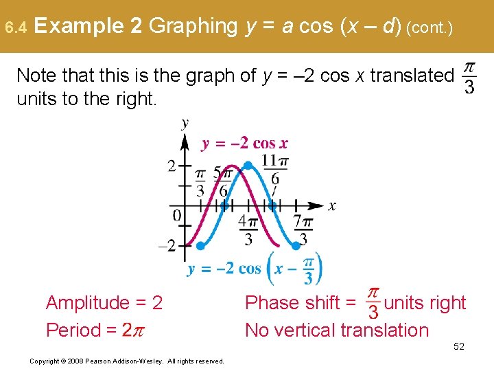
6. 4 Example 2 Graphing y = a cos (x – d) (cont. ) Note that this is the graph of y = – 2 cos x translated units to the right. Amplitude = 2 Period = Phase shift = units right No vertical translation 52 Copyright © 2008 Pearson Addison-Wesley. All rights reserved.

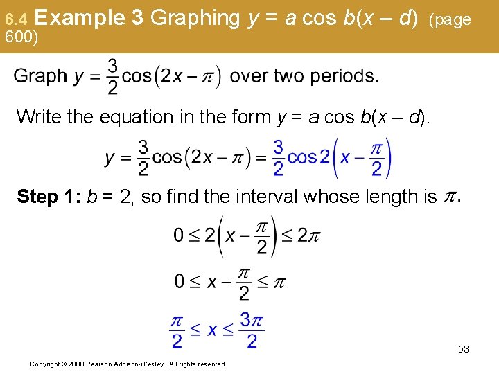
6. 4 Example 600) 3 Graphing y = a cos b(x – d) (page Write the equation in the form y = a cos b(x – d). Step 1: b = 2, so find the interval whose length is 53 Copyright © 2008 Pearson Addison-Wesley. All rights reserved.

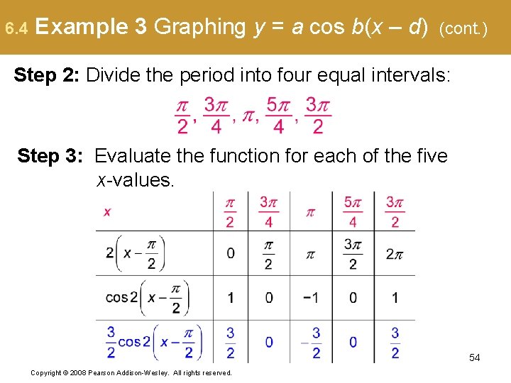
6. 4 Example 3 Graphing y = a cos b(x – d) (cont. ) Step 2: Divide the period into four equal intervals: Step 3: Evaluate the function for each of the five x-values. 54 Copyright © 2008 Pearson Addison-Wesley. All rights reserved.

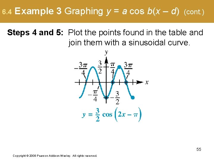
6. 4 Example 3 Graphing y = a cos b(x – d) (cont. ) Steps 4 and 5: Plot the points found in the table and join them with a sinusoidal curve. 55 Copyright © 2008 Pearson Addison-Wesley. All rights reserved.

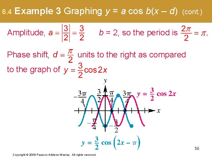
6. 4 Example 3 Graphing y = a cos b(x – d) Amplitude, Phase shift, (cont. ) b = 2, so the period is units to the right as compared to the graph of 56 Copyright © 2008 Pearson Addison-Wesley. All rights reserved.

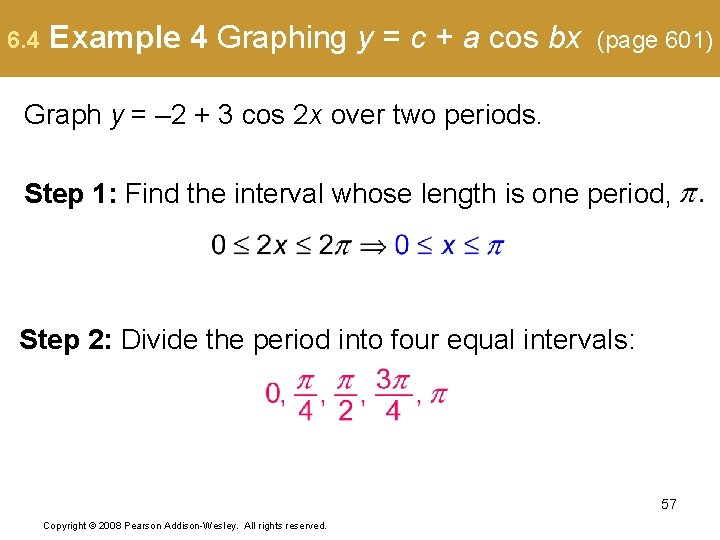
6. 4 Example 4 Graphing y = c + a cos bx (page 601) Graph y = – 2 + 3 cos 2 x over two periods. Step 1: Find the interval whose length is one period, Step 2: Divide the period into four equal intervals: 57 Copyright © 2008 Pearson Addison-Wesley. All rights reserved.

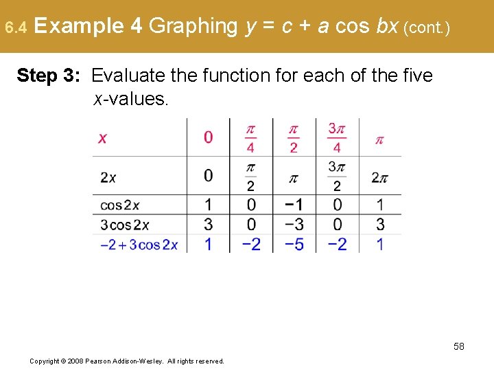
6. 4 Example 4 Graphing y = c + a cos bx (cont. ) Step 3: Evaluate the function for each of the five x-values. 58 Copyright © 2008 Pearson Addison-Wesley. All rights reserved.

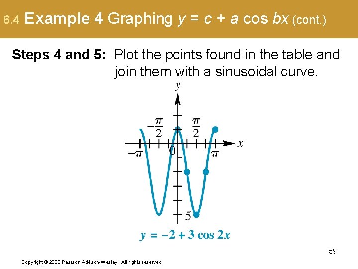
6. 4 Example 4 Graphing y = c + a cos bx (cont. ) Steps 4 and 5: Plot the points found in the table and join them with a sinusoidal curve. 59 Copyright © 2008 Pearson Addison-Wesley. All rights reserved.

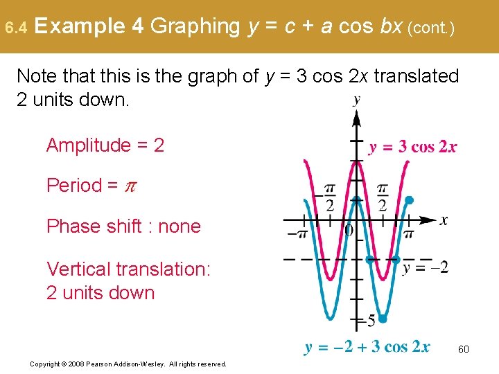
6. 4 Example 4 Graphing y = c + a cos bx (cont. ) Note that this is the graph of y = 3 cos 2 x translated 2 units down. Amplitude = 2 Period = Phase shift : none Vertical translation: 2 units down 60 Copyright © 2008 Pearson Addison-Wesley. All rights reserved.

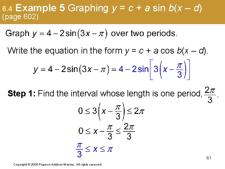
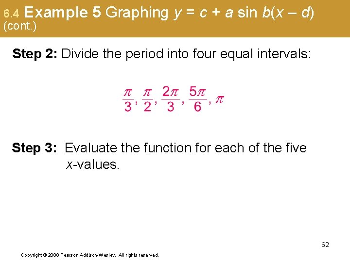
6. 4 Example (page 602) 5 Graphing y = c + a sin b(x – d) Write the equation in the form y = c + a cos b(x – d). Step 1: Find the interval whose length is one period, 61 Copyright © 2008 Pearson Addison-Wesley. All rights reserved.

6. 4 Example (cont. ) 5 Graphing y = c + a sin b(x – d) Step 2: Divide the period into four equal intervals: Step 3: Evaluate the function for each of the five x-values. 62 Copyright © 2008 Pearson Addison-Wesley. All rights reserved.

6. 4 Example (cont. ) 5 Graphing y = c + a sin b(x – d) 63 Copyright © 2008 Pearson Addison-Wesley. All rights reserved.

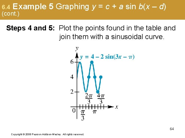
6. 4 Example (cont. ) 5 Graphing y = c + a sin b(x – d) Steps 4 and 5: Plot the points found in the table and join them with a sinusoidal curve. 64 Copyright © 2008 Pearson Addison-Wesley. All rights reserved.

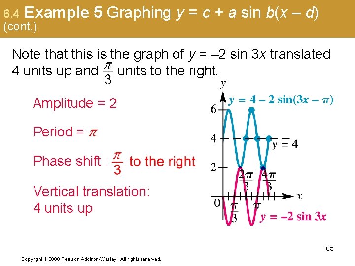
6. 4 Example (cont. ) 5 Graphing y = c + a sin b(x – d) Note that this is the graph of y = – 2 sin 3 x translated 4 units up and units to the right. Amplitude = 2 Period = Phase shift : Vertical translation: 4 units up 65 Copyright © 2008 Pearson Addison-Wesley. All rights reserved.

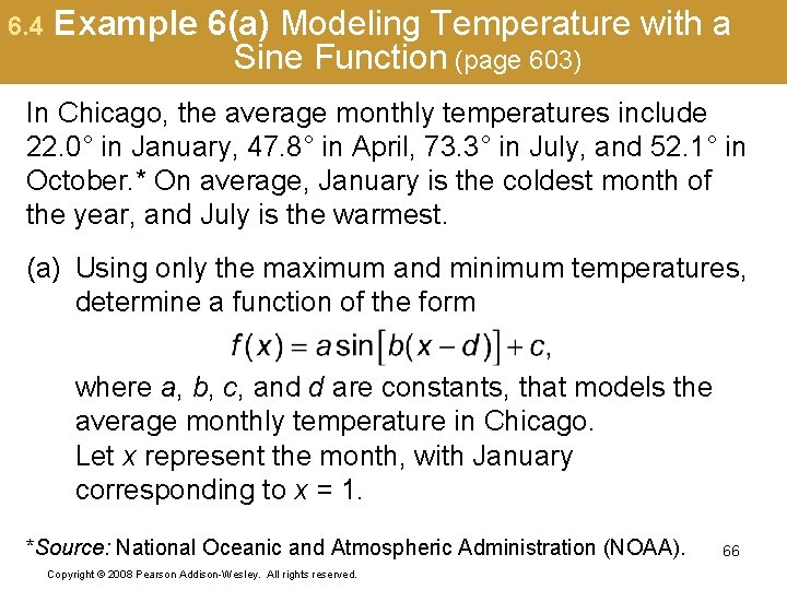
6. 4 Example 6(a) Modeling Temperature with a Sine Function (page 603) In Chicago, the average monthly temperatures include 22. 0° in January, 47. 8° in April, 73. 3° in July, and 52. 1° in October. * On average, January is the coldest month of the year, and July is the warmest. (a) Using only the maximum and minimum temperatures, determine a function of the form where a, b, c, and d are constants, that models the average monthly temperature in Chicago. Let x represent the month, with January corresponding to x = 1. *Source: National Oceanic and Atmospheric Administration (NOAA). Copyright © 2008 Pearson Addison-Wesley. All rights reserved. 66

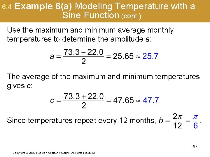
6. 4 Example 6(a) Modeling Temperature with a Sine Function (cont. ) Use the maximum and minimum average monthly temperatures to determine the amplitude a: The average of the maximum and minimum temperatures gives c: Since temperatures repeat every 12 months, 67 Copyright © 2008 Pearson Addison-Wesley. All rights reserved.

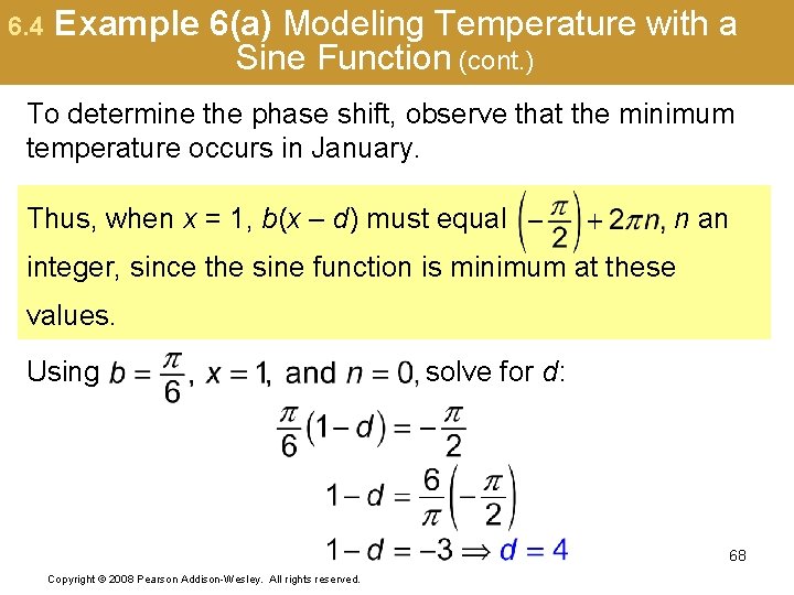
6. 4 Example 6(a) Modeling Temperature with a Sine Function (cont. ) To determine the phase shift, observe that the minimum temperature occurs in January. Thus, when x = 1, b(x – d) must equal n an integer, since the sine function is minimum at these values. Using solve for d: 68 Copyright © 2008 Pearson Addison-Wesley. All rights reserved.

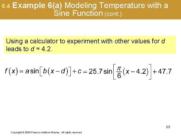
6. 4 Example 6(a) Modeling Temperature with a Sine Function (cont. ) Using a calculator to experiment with other values for d leads to d ≈ 4. 2. 69 Copyright © 2008 Pearson Addison-Wesley. All rights reserved.

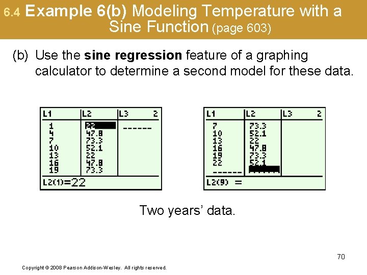
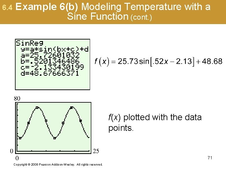
6. 4 Example 6(b) Modeling Temperature with a Sine Function (page 603) (b) Use the sine regression feature of a graphing calculator to determine a second model for these data. Two years’ data. 70 Copyright © 2008 Pearson Addison-Wesley. All rights reserved.

6. 4 Example 6(b) Modeling Temperature with a Sine Function (cont. ) f(x) plotted with the data points. 71 Copyright © 2008 Pearson Addison-Wesley. All rights reserved.

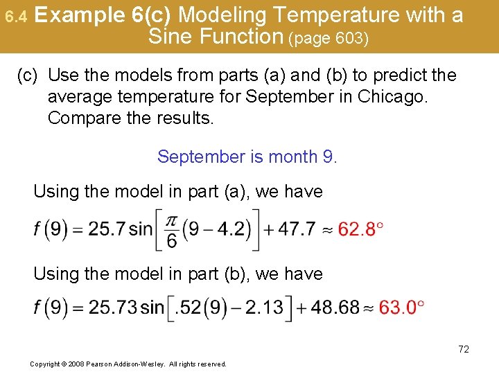
6. 4 Example 6(c) Modeling Temperature with a Sine Function (page 603) (c) Use the models from parts (a) and (b) to predict the average temperature for September in Chicago. Compare the results. September is month 9. Using the model in part (a), we have Using the model in part (b), we have 72 Copyright © 2008 Pearson Addison-Wesley. All rights reserved.