6 Ordered Choice Models Ordered Choices Ordered Discrete

6. Ordered Choice Models

Ordered Choices

Ordered Discrete Outcomes • • E. g. : Taste test, credit rating, course grade, preference scale Underlying random preferences: • • • Existence of an underlying continuous preference scale Mapping to observed choices Strength of preferences is reflected in the discrete outcome Censoring and discrete measurement The nature of ordered data

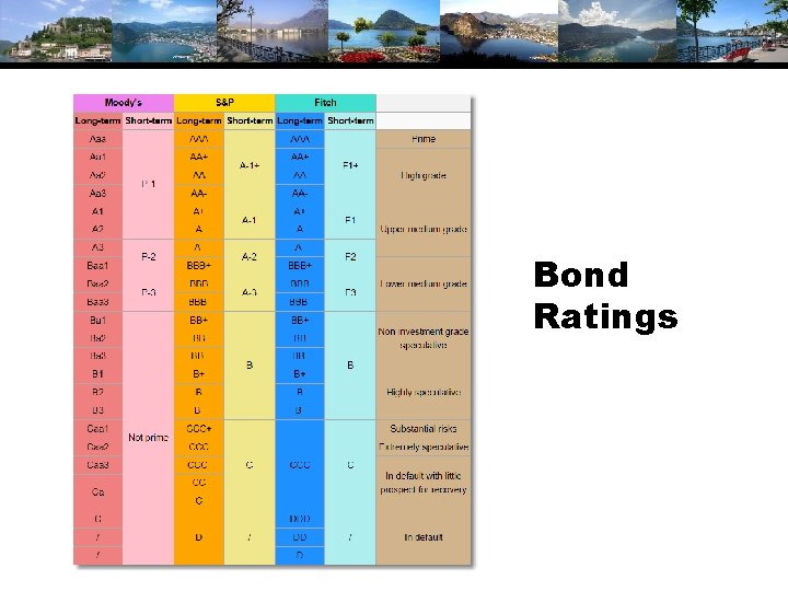
Bond Ratings

Health Satisfaction (HSAT) Self administered survey: Health Satisfaction (0 – 10) Continuous Preference Scale

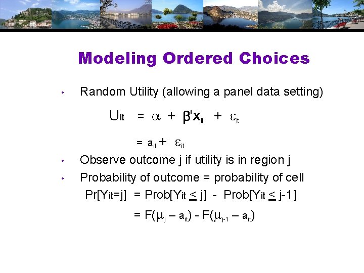
Modeling Ordered Choices • Random Utility (allowing a panel data setting) Uit = + 'xit + it = ait + • • it Observe outcome j if utility is in region j Probability of outcome = probability of cell Pr[Yit=j] = Prob[Yit < j] - Prob[Yit < j-1] = F( j – ait) - F( j-1 – ait)

Ordered Probability Model

Combined Outcomes for Health Satisfaction

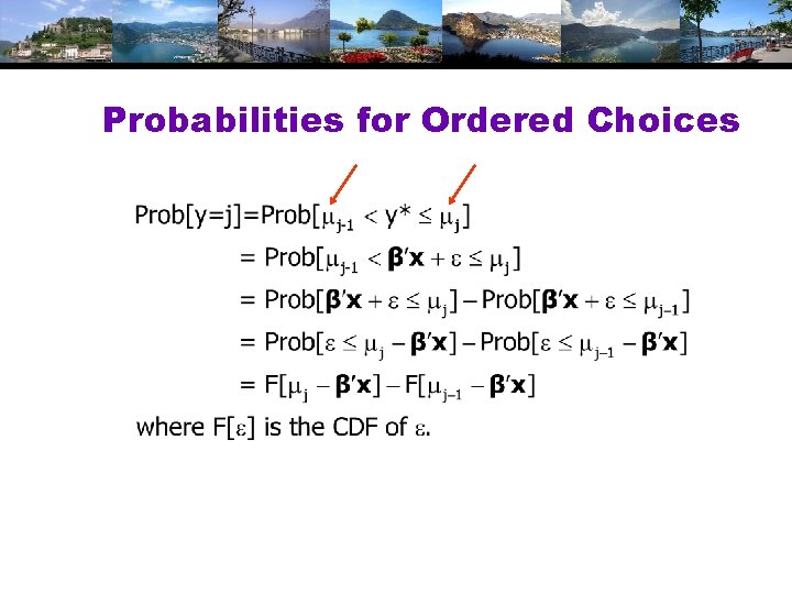
Probabilities for Ordered Choices

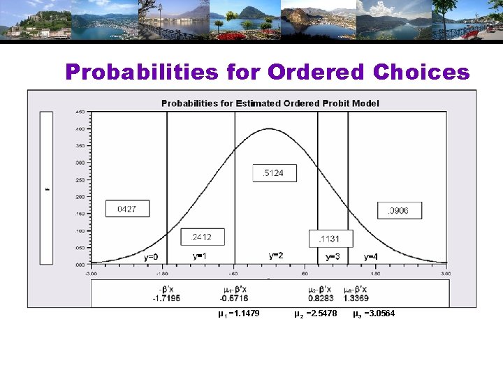
Probabilities for Ordered Choices μ 1 =1. 1479 μ 2 =2. 5478 μ 3 =3. 0564

Coefficients

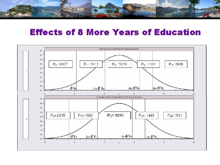
Effects of 8 More Years of Education

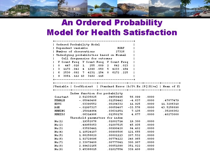
An Ordered Probability Model for Health Satisfaction +-----------------------+ | Ordered Probability Model | | Dependent variable HSAT | | Number of observations 27326 | | Underlying probabilities based on Normal | | Cell frequencies for outcomes | | Y Count Freq | | 0 447. 016 1 255. 009 2 642. 023 | | 3 1173. 042 4 1390. 050 5 4233. 154 | | 6 2530. 092 7 4231. 154 8 6172. 225 | | 9 3061. 112 10 3192. 116 | +-----------------------+ +--------------+--------+---------+-----+ |Variable | Coefficient | Standard Error |b/St. Er. |P[|Z|>z] | Mean of X| +--------------+--------+---------+-----+ Index function for probability Constant 2. 61335825. 04658496 56. 099. 0000 FEMALE -. 05840486. 01259442 -4. 637. 0000. 47877479 EDUC. 03390552. 00284332 11. 925. 0000 11. 3206310 AGE -. 01997327. 00059487 -33. 576. 0000 43. 5256898 HHNINC. 25914964. 03631951 7. 135. 0000. 35208362 HHKIDS. 06314906. 01350176 4. 677. 0000. 40273000 Threshold parameters for index Mu(1). 19352076. 01002714 19. 300. 0000 Mu(2). 49955053. 01087525 45. 935. 0000 Mu(3). 83593441. 00990420 84. 402. 0000 Mu(4) 1. 10524187. 00908506 121. 655. 0000 Mu(5) 1. 66256620. 00801113 207. 532. 0000 Mu(6) 1. 92729096. 00774122 248. 965. 0000 Mu(7) 2. 33879408. 00777041 300. 987. 0000 Mu(8) 2. 99432165. 00851090 351. 822. 0000 Mu(9) 3. 45366015. 01017554 339. 408. 0000

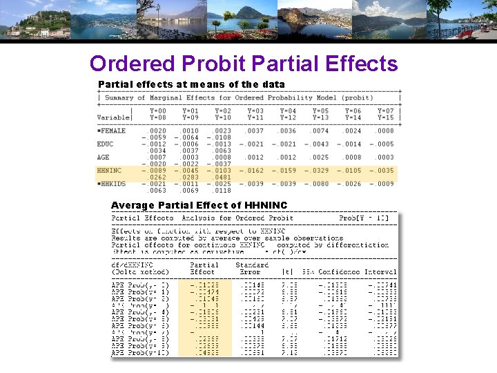
Ordered Probit Partial Effects Partial effects at means of the data Average Partial Effect of HHNINC

Fit Measures • • There is no single “dependent variable” to explain. There is no sum of squares or other measure of “variation” to explain. Predictions of the model relate to a set of J+1 probabilities, not a single variable. How to explain fit? • • • Based on the underlying regression Based on the likelihood function Based on prediction of the outcome variable

Log Likelihood Based Fit Measures

Fit Measure Based on Counting Predictions This model always predicts the same cell.

A Somewhat Better Fit

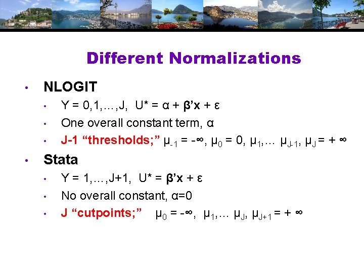
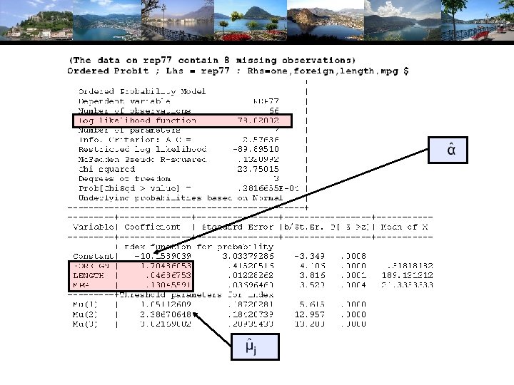
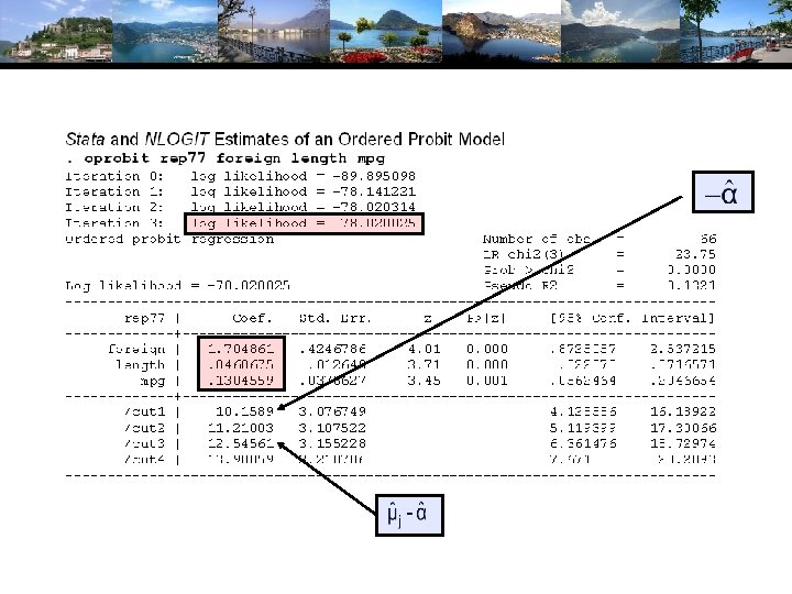
Different Normalizations • NLOGIT • • Y = 0, 1, …, J, U* = α + β’x + ε One overall constant term, α J-1 “thresholds; ” μ-1 = -∞, μ 0 = 0, μ 1, … μJ-1, μJ = + ∞ Stata • • • Y = 1, …, J+1, U* = β’x + ε No overall constant, α=0 J “cutpoints; ” μ 0 = -∞, μ 1, … μJ, μJ+1 = + ∞

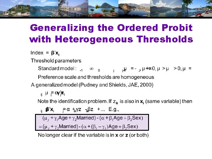
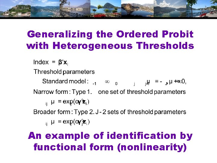
Generalizing the Ordered Probit with Heterogeneous Thresholds

Generalizing the Ordered Probit with Heterogeneous Thresholds An example of identification by functional form (nonlinearity)

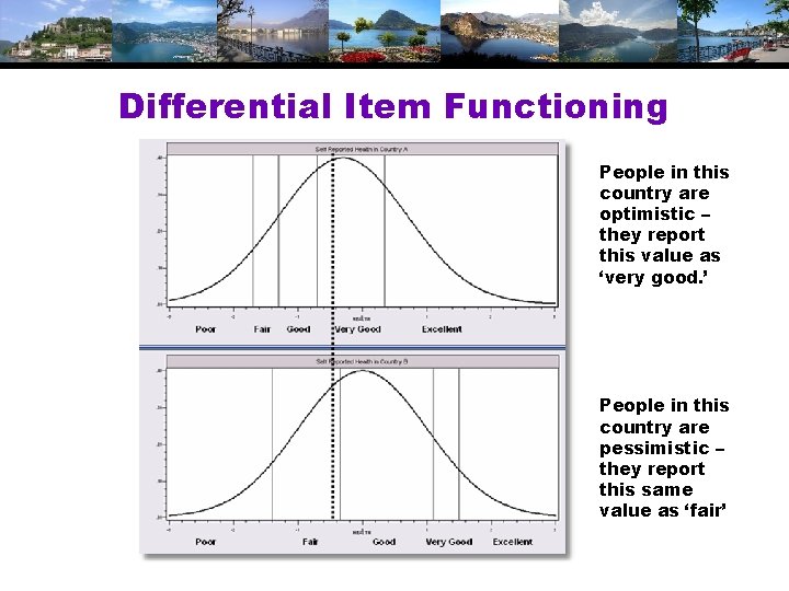
Differential Item Functioning People in this country are optimistic – they report this value as ‘very good. ’ People in this country are pessimistic – they report this same value as ‘fair’

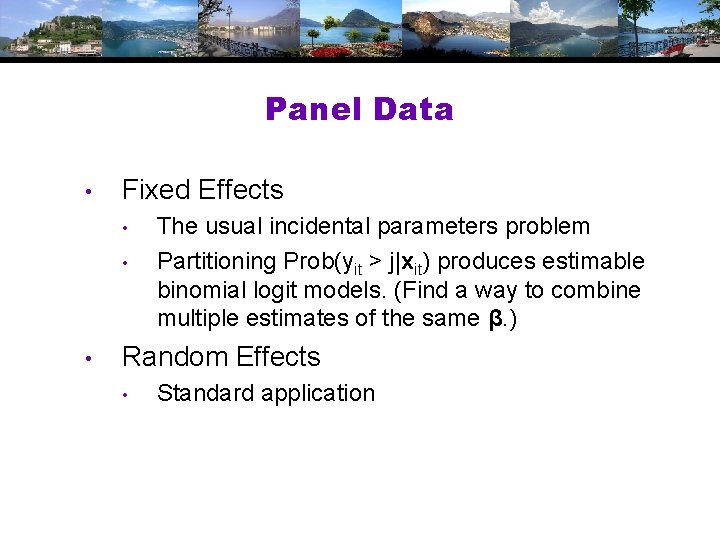
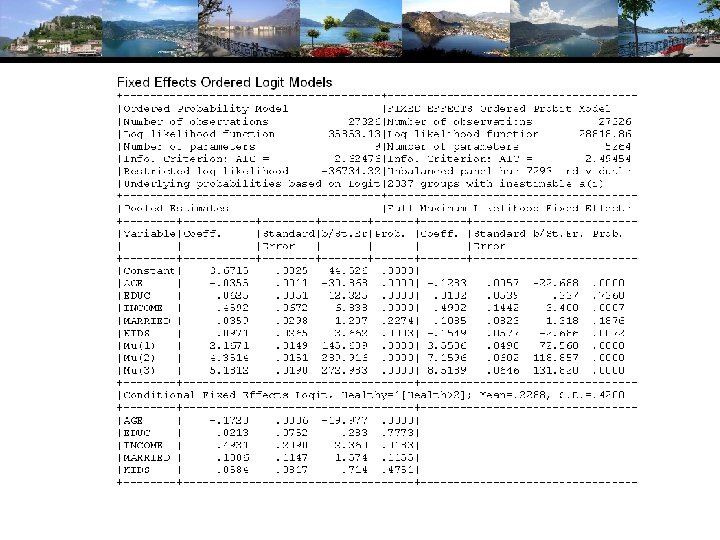
Panel Data • Fixed Effects • • • The usual incidental parameters problem Partitioning Prob(yit > j|xit) produces estimable binomial logit models. (Find a way to combine multiple estimates of the same β. ) Random Effects • Standard application

Incidental Parameters Problem Monte Carlo Analysis of the Bias of the MLE in Fixed Effects Discrete Choice Models (Means of empirical sampling distributions, N = 1, 000 individuals, R = 200 replications)

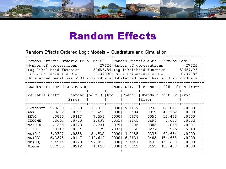
Random Effects

Dynamic Ordered Probit Model

Model for Self Assessed Health • British Household Panel Survey (BHPS) • • • Waves 1 -8, 1991 -1998 Self assessed health on 0, 1, 2, 3, 4 scale Sociological and demographic covariates Dynamics – inertia in reporting of top scale Dynamic ordered probit model • • Balanced panel – analyze dynamics Unbalanced panel – examine attrition

Dynamic Ordered Probit Model It would not be appropriate to include hi, t-1 itself in the model as this is a label, not a measure

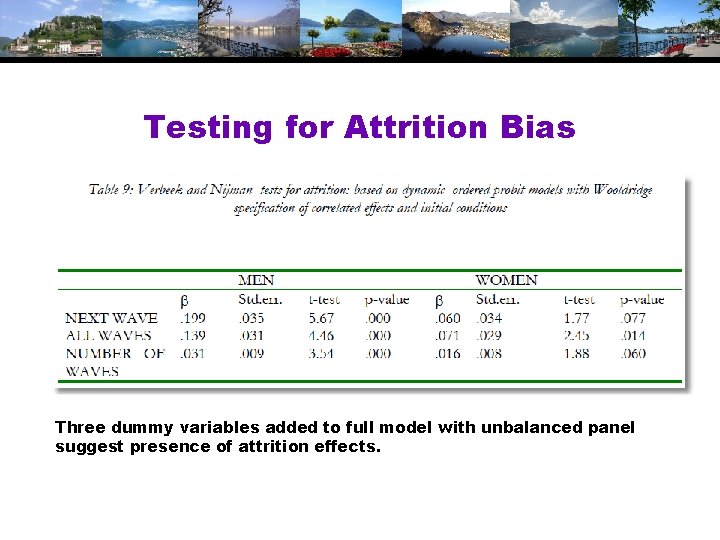
Testing for Attrition Bias Three dummy variables added to full model with unbalanced panel suggest presence of attrition effects.

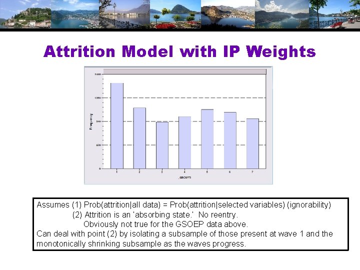
Attrition Model with IP Weights Assumes (1) Prob(attrition|all data) = Prob(attrition|selected variables) (ignorability) (2) Attrition is an ‘absorbing state. ’ No reentry. Obviously not true for the GSOEP data above. Can deal with point (2) by isolating a subsample of those present at wave 1 and the monotonically shrinking subsample as the waves progress.

Inverse Probability Weighting

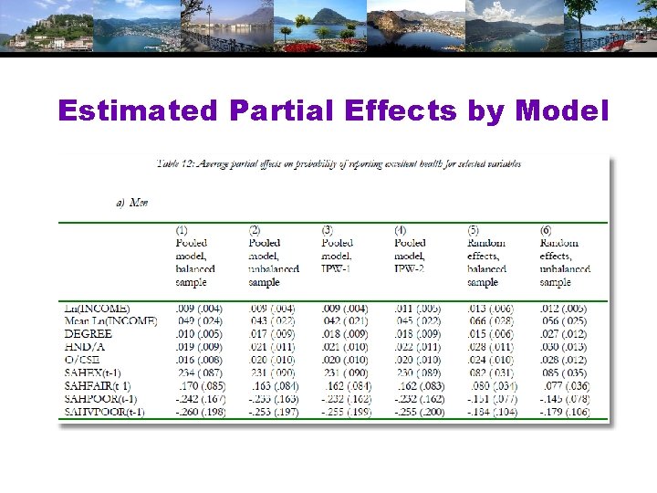
Estimated Partial Effects by Model

Partial Effect for a Category These are 4 dummy variables for state in the previous period. Using first differences, the 0. 234 estimated for SAHEX means transition from EXCELLENT in the previous period to GOOD in the previous period, where GOOD is the omitted category. Likewise for the other 3 previous state variables. The margin from ‘POOR’ to ‘GOOD’ was not interesting in the paper. The better margin would have been from EXCELLENT to POOR, which would have (EX, POOR) change from (1, 0) to (0, 1).