6 Model Structures 1 ARX model structure In

(6) Model Structures 1

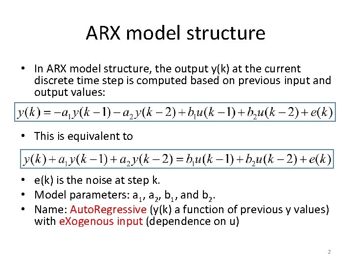
ARX model structure • In ARX model structure, the output y(k) at the current discrete time step is computed based on previous input and output values: • This is equivalent to • e(k) is the noise at step k. • Model parameters: a 1, a 2, b 1, and b 2. • Name: Auto. Regressive (y(k) a function of previous y values) with e. Xogenous input (dependence on u) 2

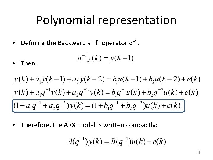
Polynomial representation • Defining the Backward shift operator q− 1: • Then: • Therefore, the ARX model is written compactly: 3

Remarks • Usually, the ARX model is the first model to try in system identification. • The ARX model is quite general, it can describe arbitrary linear relationships between inputs and outputs. • However, the noise enters the model in a restricted way, and later we introduce models that generalize this. 4

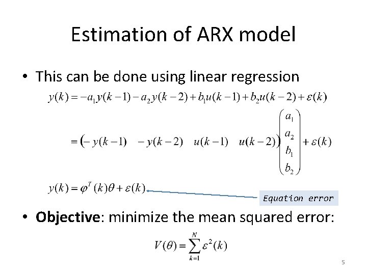
Estimation of ARX model • This can be done using linear regression Equation error • Objective: minimize the mean squared error: 5

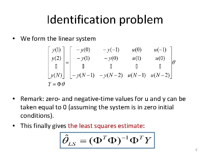
Identification problem • We form the linear system • Remark: zero- and negative-time values for u and y can be taken equal to 0 (assuming the system is in zero initial conditions). • This finally gives the least squares estimate: 6

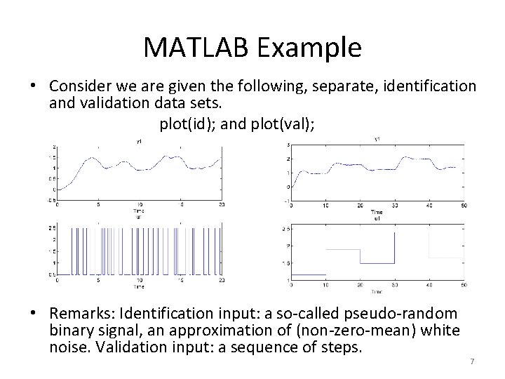
MATLAB Example • Consider we are given the following, separate, identification and validation data sets. plot(id); and plot(val); • Remarks: Identification input: a so-called pseudo-random binary signal, an approximation of (non-zero-mean) white noise. Validation input: a sequence of steps. 7

Identifying an ARX model = arx(id, [na, nb, nk]); • Arguments: 1 - Identification data. 2 - Array containing the orders of A and B and the delay nk. 8

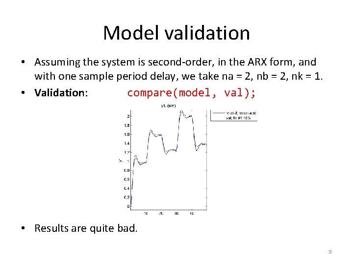
Model validation • Assuming the system is second-order, in the ARX form, and with one sample period delay, we take na = 2, nb = 2, nk = 1. • Validation: compare(model, val); • Results are quite bad. 9

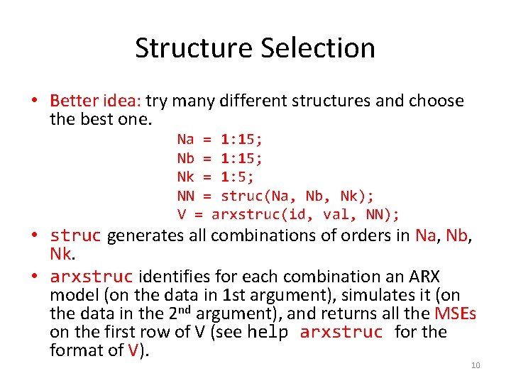
Structure Selection • Better idea: try many different structures and choose the best one. Na = 1: 15; Nb = 1: 15; Nk = 1: 5; NN = struc(Na, Nb, Nk); V = arxstruc(id, val, NN); • struc generates all combinations of orders in Na, Nb, Nk. • arxstruc identifies for each combination an ARX model (on the data in 1 st argument), simulates it (on the data in the 2 nd argument), and returns all the MSEs on the first row of V (see help arxstruc for the format of V). 10

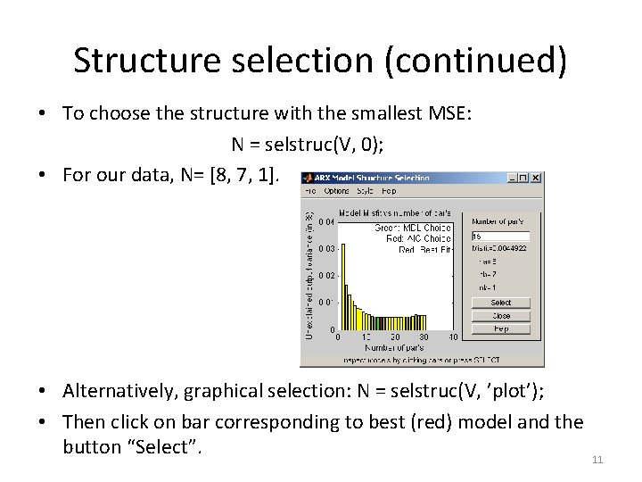
Structure selection (continued) • To choose the structure with the smallest MSE: N = selstruc(V, 0); • For our data, N= [8, 7, 1]. • Alternatively, graphical selection: N = selstruc(V, ’plot’); • Then click on bar corresponding to best (red) model and the button “Select”. 11

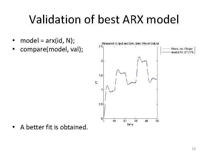
Validation of best ARX model • model = arx(id, N); • compare(model, val); • A better fit is obtained. 12

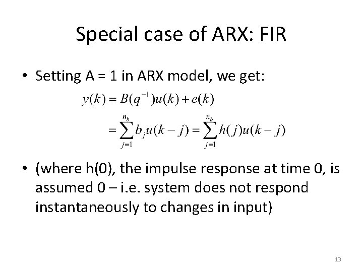
Special case of ARX: FIR • Setting A = 1 in ARX model, we get: • (where h(0), the impulse response at time 0, is assumed 0 – i. e. system does not respond instantaneously to changes in input) 13

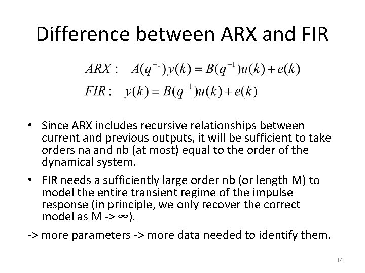
Difference between ARX and FIR • Since ARX includes recursive relationships between current and previous outputs, it will be sufficient to take orders na and nb (at most) equal to the order of the dynamical system. • FIR needs a sufficiently large order nb (or length M) to model the entire transient regime of the impulse response (in principle, we only recover the correct model as M -> ∞). -> more parameters -> more data needed to identify them. 14

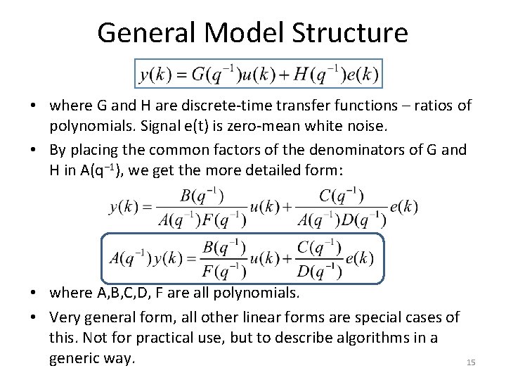
General Model Structure • where G and H are discrete-time transfer functions – ratios of polynomials. Signal e(t) is zero-mean white noise. • By placing the common factors of the denominators of G and H in A(q− 1), we get the more detailed form: • where A, B, C, D, F are all polynomials. • Very general form, all other linear forms are special cases of this. Not for practical use, but to describe algorithms in a generic way. 15

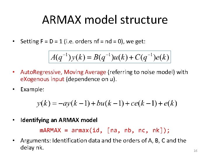
ARMAX model structure • Setting F = D = 1 (i. e. orders nf = nd = 0), we get: • Auto. Regressive, Moving Average (referring to noise model) with e. Xogenous input (dependence on u). • Example: • Identifying an ARMAX model m. ARMAX = armax(id, [na, nb, nc, nk]); • Arguments: Identification data and the orders of A, B, C and the delay nk. 16

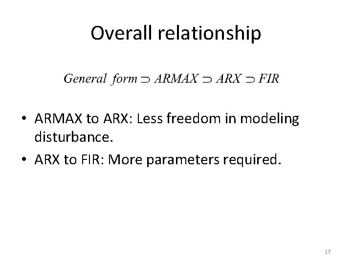
Overall relationship • ARMAX to ARX: Less freedom in modeling disturbance. • ARX to FIR: More parameters required. 17

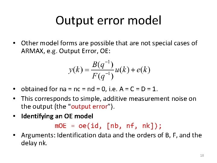
Output error model • Other model forms are possible that are not special cases of ARMAX, e. g. Output Error, OE: • obtained for na = nc = nd = 0, i. e. A = C = D = 1. • This corresponds to simple, additive measurement noise on the output (the “output error”). • Identifying an OE model m. OE = oe(id, [nb, nf, nk]); • Arguments: Identification data and the orders of B, F, and the delay nk. 18