6 INCREASING RETURNS TO SCALE AND IMPERFECT COMPETITION

• 6 INCREASING RETURNS TO SCALE AND IMPERFECT COMPETITION 1 Basics of Imperfect Competition 2 Trade under Monopolistic Competition 3 Empirical Applications of Monopolistic Competition and Trade 4 Imperfect Competition with Homogeneous Products 5 Conclusions

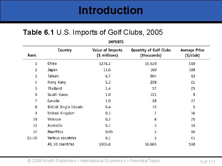
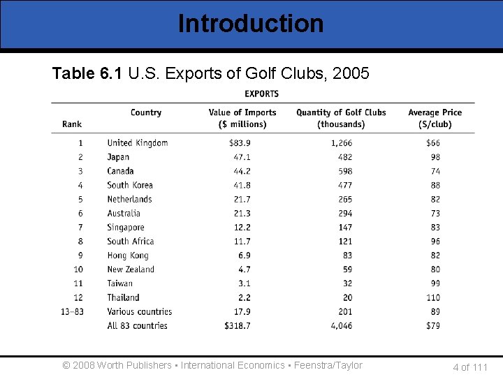
Introduction • We will look at trade in golf clubs, a good that the U. S. imports and exports in large quantities. • Many countries that sell to the U. S. are also buying from the U. S. w The total value of imports is close to the total value of exports. • Why does the U. S. export and import golf clubs to and from the same countries? w We observe intra-industry trade. w A new explanation for trade will be discussed here. © 2008 Worth Publishers ▪ International Economics ▪ Feenstra/Taylor 2 of 111

Introduction Table 6. 1 U. S. Imports of Golf Clubs, 2005 © 2008 Worth Publishers ▪ International Economics ▪ Feenstra/Taylor 3 of 111

Introduction Table 6. 1 U. S. Exports of Golf Clubs, 2005 © 2008 Worth Publishers ▪ International Economics ▪ Feenstra/Taylor 4 of 111

Introduction • We will look at a model of monopolistic competition where goods are differentiated. w Gives a degree of market power • Firms tend to specialize because in monopolistic competition we have increasing returns to scale • The imperfect competition model also predicts that larger countries will trade more with each other. w This is called the gravity equation. © 2008 Worth Publishers ▪ International Economics ▪ Feenstra/Taylor 5 of 111

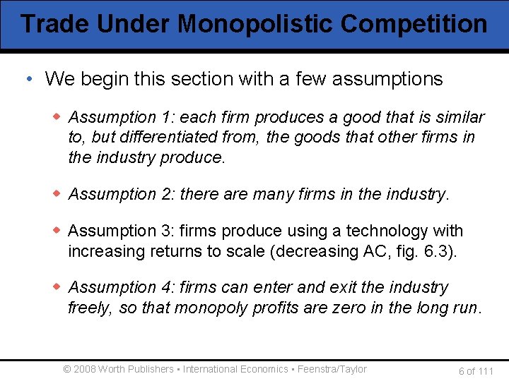
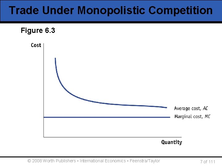
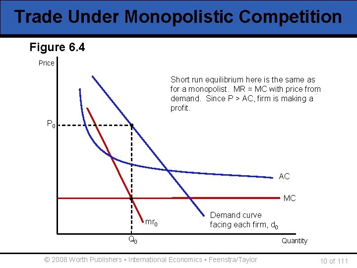
Trade Under Monopolistic Competition • We begin this section with a few assumptions w Assumption 1: each firm produces a good that is similar to, but differentiated from, the goods that other firms in the industry produce. w Assumption 2: there are many firms in the industry. w Assumption 3: firms produce using a technology with increasing returns to scale (decreasing AC, fig. 6. 3). w Assumption 4: firms can enter and exit the industry freely, so that monopoly profits are zero in the long run. © 2008 Worth Publishers ▪ International Economics ▪ Feenstra/Taylor 6 of 111

Trade Under Monopolistic Competition Figure 6. 3 © 2008 Worth Publishers ▪ International Economics ▪ Feenstra/Taylor 7 of 111

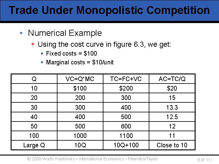
Trade Under Monopolistic Competition • Numerical Example w Using the cost curve in figure 6. 3, we get: § Fixed costs = $100 § Marginal costs = $10/unit Q VC=Q*MC TC=FC+VC AC=TC/Q 10 $100 $20 20 200 300 15 30 300 400 13. 3 40 400 500 12. 5 50 500 600 12 1000 1100 11 Large Q 10 Q+100 Close to 10 © 2008 Worth Publishers ▪ International Economics ▪ Feenstra/Taylor 8 of 111

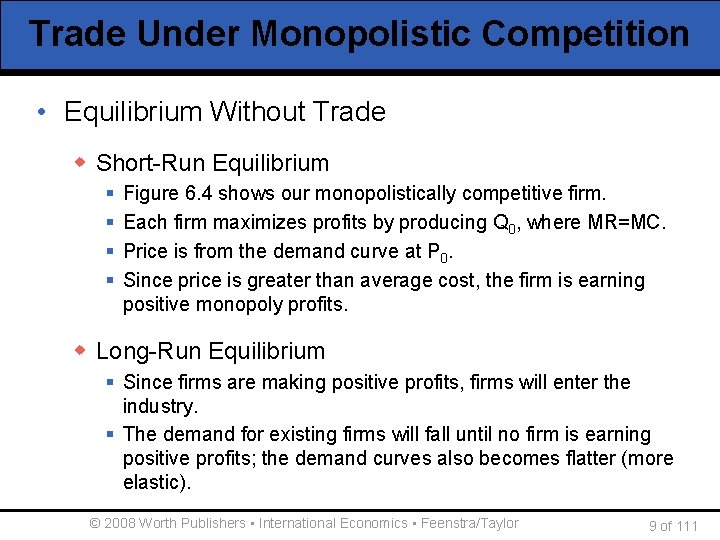
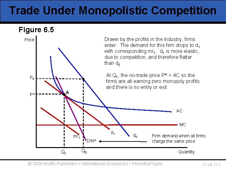
Trade Under Monopolistic Competition • Equilibrium Without Trade w Short-Run Equilibrium § § Figure 6. 4 shows our monopolistically competitive firm. Each firm maximizes profits by producing Q 0, where MR=MC. Price is from the demand curve at P 0. Since price is greater than average cost, the firm is earning positive monopoly profits. w Long-Run Equilibrium § Since firms are making positive profits, firms will enter the industry. § The demand for existing firms will fall until no firm is earning positive profits; the demand curves also becomes flatter (more elastic). © 2008 Worth Publishers ▪ International Economics ▪ Feenstra/Taylor 9 of 111

Trade Under Monopolistic Competition Figure 6. 4 Price Short run equilibrium here is the same as for a monopolist. MR = MC with price from demand. Since P > AC, firm is making a profit. P 0 AC MC mr 0 Demand curve facing each firm, d 0 Q 0 © 2008 Worth Publishers ▪ International Economics ▪ Feenstra/Taylor Quantity 10 of 111

Trade Under Monopolistic Competition Figure 6. 5 Drawn by the profits in the industry, firms enter. The demand for this firm drops to d 1 Equilibrium is at A, producing Q 1, with corresponding mr 1. d 1 is more elastic, where mr 1 crosses MC. This gives due to competition, and therefore flatter price, PA, from the demand, d 1 than d 0 Price At Q 1, the no-trade price PA = AC so the firms are all earning zero monopoly profits and there is no entry or exit P 0 PA A AC MC mr 1 Q 1 d 1 D/NA d 0 Firm demand when all firms charge the same price Q 0 © 2008 Worth Publishers ▪ International Economics ▪ Feenstra/Taylor Quantity 11 of 111

Trade Under Monopolistic Competition • Equilibrium With Free Trade w Assume Home and Foreign are exactly the same. § Same number of consumers § Same technology and cost curves § Same number of firms in the no-trade equilibrium (NA) w If there were no economies of scale, there would be no reason for trade. • Short-Run Equilibrium with Trade w When trade opens, the number of customers available to each firm doubles, but the number of product varieties available to each consumer also doubles. w With the greater number of varieties available, the demand for each individual variety will be more elastic. © 2008 Worth Publishers ▪ International Economics ▪ Feenstra/Taylor 12 of 111

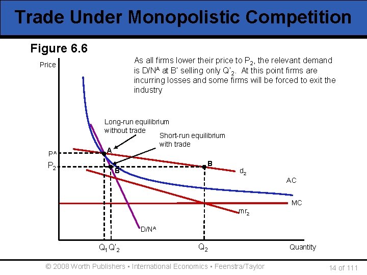
Trade Under Monopolistic Competition • Short-Run Equilibrium with Trade w After trade, demand is no longer tangent to the AC. § Each firm now produces at Q 2 charging P 2. § Firms are making positive monopoly profits. § This shows the firm’s incentive to lower its price w Every firm in the industry has the same incentive. w If all firms lower prices, though, the quantity demanded from each firm increases along D/NA, instead of d 2. § Remember D/NA is the demand if all firms had the same price. w In the short run, firms lower their prices expecting to make profits at B, but end up with losses at B′. © 2008 Worth Publishers ▪ International Economics ▪ Feenstra/Taylor 13 of 111

Trade Under Monopolistic Competition Figure 6. 6 As all firms lower their the price to Pdemand Opening trade makes firm’s even more 2, the relevant A is D/N at B’ selling Q’firm this point are at Q 2, elastic, shown by d 2 only. The chooses to firms produce 2. At incurring losses and some forced exit the where MR=MC, selling at Pfirms thisbe price the to firm makes 2. Atwill industry monopoly profits as P 2>AC Price PA P 2 Long-run equilibrium without trade Short-run equilibrium with trade A B B’ d 2 AC MC mr 2 D/NA Q 1 Q’ 2 Q 2 © 2008 Worth Publishers ▪ International Economics ▪ Feenstra/Taylor Quantity 14 of 111

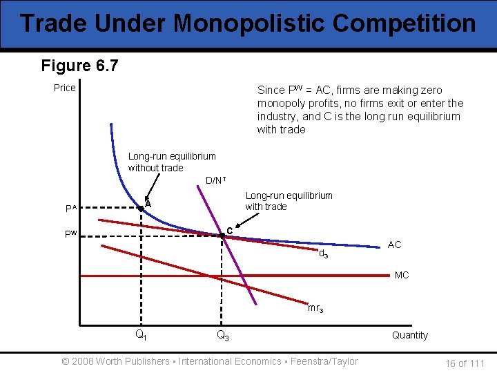
Trade Under Monopolistic Competition • Long-Run Equilibrium with Trade w Since firms will exit the industry, increasing demand for the remaining firms’ products and decrease the available product varieties to consumers. w We now only have NT firms which is fewer than the NA firms we had before. w The new demand D/NT lies to the right of D/NA. w Long-run equilibrium with trade is at point C. w The demand for each firm d 3 is tangent to AC. © 2008 Worth Publishers ▪ International Economics ▪ Feenstra/Taylor 15 of 111

Trade Under Monopolistic Competition Figure 6. 7 Price Since some firms have exited the is Since PW = AC, firms making zero The demand faced byare each firm d 3 industry, are left T firms monopoly nowith firms exit orwhich enter the with mr 3 we. profits, mr 3=MC shows that each gives eachand firm. CQ aisshare of the Wequilibrium industry, the long rundemand firm produces 3 at a price P T shown by D/N with trade Long-run equilibrium without trade D/NT PA Long-run equilibrium with trade A C PW d 3 AC MC mr 3 Q 1 Q 3 © 2008 Worth Publishers ▪ International Economics ▪ Feenstra/Taylor Quantity 16 of 111

Trade Under Monopolistic Competition • Long-Run Equilibrium with Trade w The world number of products is greater than the number available in each country before trade. w Fewer firms remain in each country, but each is bigger. w As quantity increases, average costs fall due to increasing returns to scale, therefore so do prices. • Gains From Trade w There are two sources of gains for consumers: § Price is lower after trade. § Consumers obtain higher surplus when there are more product varieties from which to choose. © 2008 Worth Publishers ▪ International Economics ▪ Feenstra/Taylor 17 of 111

Trade Under Monopolistic Competition • Adjustment Costs from Trade w There adjustment costs as some firms shut down and exit the industry. w Workers in those firms experience a spell of unemployment. w Over the long run however, we expect those workers to find new positions. § Temporary costs w Compare short-run and long-run adjustment costs. w We will look at evidence form Mexico, Canada, and the U. S. under the North American Free Trade Agreement (NAFTA). © 2008 Worth Publishers ▪ International Economics ▪ Feenstra/Taylor 18 of 111

Empirical Applications of Monopolistic Competition and Trade • Gains and Adjustment Costs for Canada w The potential for Canadian firms to expand output was a key factor in Canada’s free-trade agreement with the U. S. in 1989 and entry into NAFTA (along with Mexico) in 1994. w Studies in Canada as early as the 1960 s predicted substantial gains from free trade with the U. S. § Firms would expand their scale of operations to service the larger market and lower their costs. w Studies by Harris in the mid-80 s influenced Canadian policy makers to proceed with the free trade agreement with the U. S. w The article described next looks at what happened in Canada after the implementation of NAFTA. © 2008 Worth Publishers ▪ International Economics ▪ Feenstra/Taylor 19 of 111

What Happened When Two countries Liberalized Trade? HEADLINES • Data from 1988– 1996 was used by Daniel Trefler of University of Toronto to estimate effects of the Canada-U. S. Free Trade Agreement. • Some findings: w Short-run adjustment costs of 100, 000 jobs, or 5% of manufacturing employment. w Some industries that had very large tariff cuts saw employment fall by as much as 12% w Over time, however, these job losses were more than made up for by creation of new jobs elsewhere in manufacturing. w There were no long run job losses due to NAFTA. © 2008 Worth Publishers ▪ International Economics ▪ Feenstra/Taylor 20 of 111

What Happened When Two countries Liberalized Trade? HEADLINES • In the long run, large positive effects on productivity were found. w 15% over eight years in industries most affected by tariff cuts— compound growth of 1. 9%/year. w 6% for manufacturing overall—compound growth of 0. 7%/year. w The difference of 1. 2%/year is an estimate of how free trade with the U. S. affected the Canadian industries over and above the impact on other industries. w There was also a rise of 3% in real earnings over this period. • These findings support the monopolistic competition model. © 2008 Worth Publishers ▪ International Economics ▪ Feenstra/Taylor 21 of 111

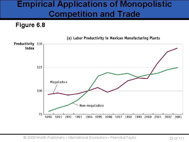
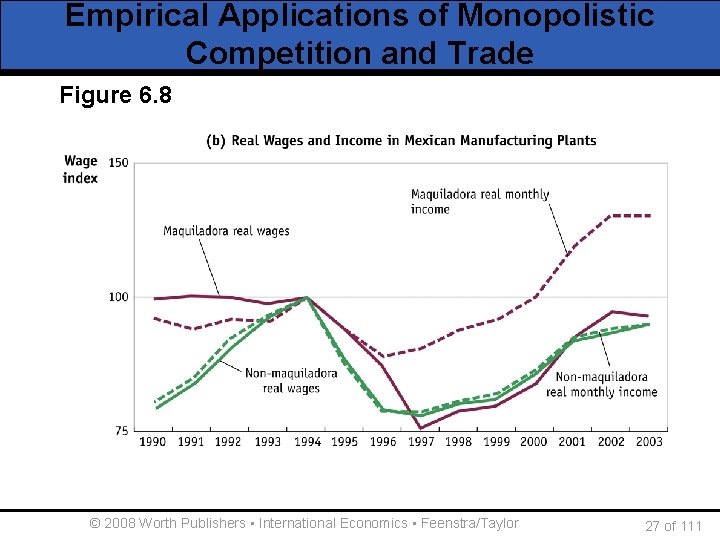
Empirical Applications of Monopolistic Competition and Trade • Gains and Adjustment Costs for Mexico w Joining NAFTA was a way to ensure the permanence of economic reforms already underway. w Under NAFTA, Mexican tariffs on U. S. goods declined from an average of 14% in 1990 to 1% in 2001. w In addition, U. S. tariffs on Mexican imports fell as well. • Productivity in Mexico (figure 6. 8) w Panel A shows productivity over time. w Panel B shows what happened to real wages and real income over time. © 2008 Worth Publishers ▪ International Economics ▪ Feenstra/Taylor 22 of 111

Empirical Applications of Monopolistic Competition and Trade Figure 6. 8 © 2008 Worth Publishers ▪ International Economics ▪ Feenstra/Taylor 23 of 111

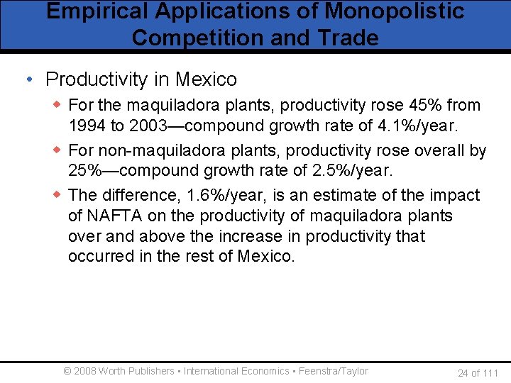
Empirical Applications of Monopolistic Competition and Trade • Productivity in Mexico w For the maquiladora plants, productivity rose 45% from 1994 to 2003—compound growth rate of 4. 1%/year. w For non-maquiladora plants, productivity rose overall by 25%—compound growth rate of 2. 5%/year. w The difference, 1. 6%/year, is an estimate of the impact of NAFTA on the productivity of maquiladora plants over and above the increase in productivity that occurred in the rest of Mexico. © 2008 Worth Publishers ▪ International Economics ▪ Feenstra/Taylor 24 of 111

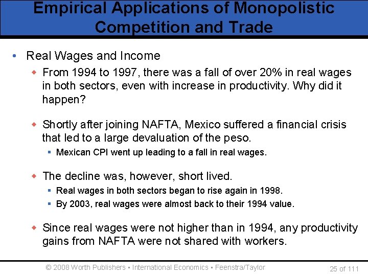
Empirical Applications of Monopolistic Competition and Trade • Real Wages and Income w From 1994 to 1997, there was a fall of over 20% in real wages in both sectors, even with increase in productivity. Why did it happen? w Shortly after joining NAFTA, Mexico suffered a financial crisis that led to a large devaluation of the peso. § Mexican CPI went up leading to a fall in real wages. w The decline was, however, short lived. § Real wages in both sectors began to rise again in 1998. § By 2003, real wages were almost back to their 1994 value. w Since real wages were not higher than in 1994, any productivity gains from NAFTA were not shared with workers. © 2008 Worth Publishers ▪ International Economics ▪ Feenstra/Taylor 25 of 111

Empirical Applications of Monopolistic Competition and Trade • Real Wages and Income w If we look at real monthly income, the picture is a little better. § This includes other sources of income beside wages, especially for higher-income persons. w In the maquiladora sector, real incomes were higher in 2003 than in 1994. § Some gains for workers in plants most affected by NAFTA. w Higher-income workers fared better than unskilled workers in Mexico. § Higher-income workers in the maquiladora sector are principal gainers due to NAFTA in the long run. © 2008 Worth Publishers ▪ International Economics ▪ Feenstra/Taylor 26 of 111

Empirical Applications of Monopolistic Competition and Trade Figure 6. 8 © 2008 Worth Publishers ▪ International Economics ▪ Feenstra/Taylor 27 of 111

Empirical Applications of Monopolistic Competition and Trade • Adjustment Costs in Mexico w When Mexico joined NAFTA, it was expected that the agricultural sector would fare the worst due to competition from the U. S. § Tariff reductions in agriculture were phased in over 15 years. w The evidence to date shows the corn farmers did not suffer as much as was feared. Why? § The poorest farmers consume the corn they grow. § Mexican government was able to use subsidies to offset the reduction in income for other corn farmers. w Total production of corn in Mexico rose following NAFTA. © 2008 Worth Publishers ▪ International Economics ▪ Feenstra/Taylor 28 of 111

Empirical Applications of Monopolistic Competition and Trade • Adjustment Costs in Mexico w Increasing volatility due to trade can be counted as adjustment costs. w For maquiladora plants, employment grew rapidly following NAFTA to a peak of 1. 29 million in 2000. w After that, this sector entered a downturn. § The U. S. entered a recession decreasing demand for Mexican exports. § China was competing for U. S. sales by exporting goods similar to those sold by Mexico. § The Mexican peso became over-valued, making it difficult to export abroad. w Employment in the maquiladora sector fell after 2000 to 1. 1 million in 2003. © 2008 Worth Publishers ▪ International Economics ▪ Feenstra/Taylor 29 of 111

Empirical Applications of Monopolistic Competition and Trade • Gains and Adjustment Costs for the U. S. w Studies on the effects of NAFTA on the U. S. have not estimated its effects on the productivity of U. S. firms. § It would be hard to identify the impact since Mexico and Canada are only two of many trading partners. w Instead, researchers have estimated the second source of gains from trade: the expansion of import varieties available to consumers. w For U. S. we will compare the long-run gains to consumers due to expanded product varieties with the short-run adjustment costs from exiting firms and unemployment. © 2008 Worth Publishers ▪ International Economics ▪ Feenstra/Taylor 30 of 111

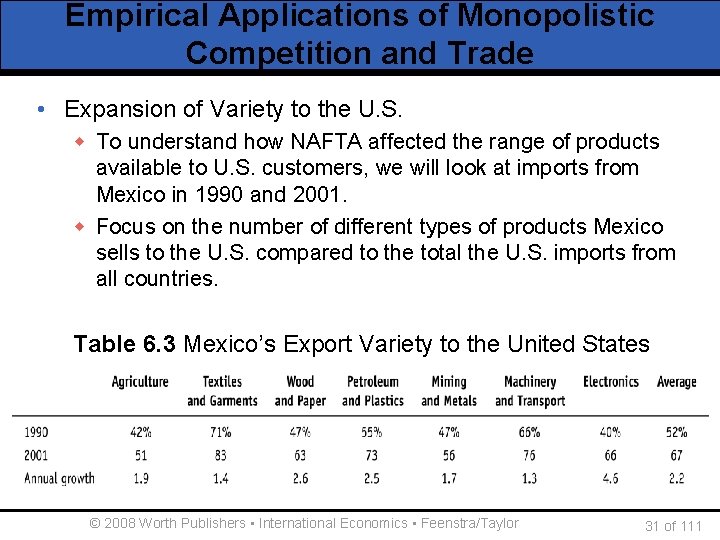
Empirical Applications of Monopolistic Competition and Trade • Expansion of Variety to the U. S. w To understand how NAFTA affected the range of products available to U. S. customers, we will look at imports from Mexico in 1990 and 2001. w Focus on the number of different types of products Mexico sells to the U. S. compared to the total the U. S. imports from all countries. Table 6. 3 Mexico’s Export Variety to the United States © 2008 Worth Publishers ▪ International Economics ▪ Feenstra/Taylor 31 of 111

Empirical Applications of Monopolistic Competition and Trade • Expansion of Variety to the U. S. w According to one estimate, the total number of product varieties imported into the U. S. from 1972– 2001 has increased four times. w That expansion in import variety has had the same effect as a reduction in import prices of 1. 2% per year. w Using an average $90 billion in U. S. imports per year and the 1. 2% reduction in prices to U. S. consumers, $90(1. 2%) = $1. 1 billion per year in savings to consumers. w These consumer savings are permanent and increase over time as export varieties grow. w In 2003, the 10 th year of NAFTA, consumers would gain $11 billion as compared to 1994. © 2008 Worth Publishers ▪ International Economics ▪ Feenstra/Taylor 32 of 111

Empirical Applications of Monopolistic Competition and Trade • Adjustment Costs in the U. S. w These come as firms exit the market due to import competition and the workers employed there are temporarily unemployed. w One way to measure this loss is to look at claims under the U. S. Trade Adjustment Assistance (TAA) provisions. w From 1994– 2002, about 525, 000 workers, or about 58, 000 per year, lost their jobs and were certified as adversely affected by trade under the NAFTA-TAA program. w Compare to the annual number of workers displaced in manufacturing or 444, 000 workers per year. w The NAFTA layoffs of 58, 000 workers were about 13% of total displacement—this is a substantial amount. © 2008 Worth Publishers ▪ International Economics ▪ Feenstra/Taylor 33 of 111

Empirical Applications of Monopolistic Competition and Trade • Adjustment Costs in the U. S. w Another way to measure effects is to compare the loss in wages from the displaced workers to the consumer gains. w Suppose the average length of unemployment for laid off workers is 3 years. w Average yearly earnings for manufacturing workers was $31, 000 in 2000 so each displaced worker lost $93, 000 in wages. total losses were $5. 4 billion. w These private costs of $5. 4 billion are nearly equal to the average welfare gains of $5. 5 billion. w However, gains continue to grow over time and job loss was only temporary. © 2008 Worth Publishers ▪ International Economics ▪ Feenstra/Taylor 34 of 111

Empirical Applications of Monopolistic Competition and Trade • Summary of NAFTA w We have been able to measure in part the long-run gains and short-run costs from NAFTA for Canada, Mexico, and the U. S. w It is clear that for Canada and the U. S. , the long-run gains considerably exceed the short-run costs. w In Mexico the gains have not been reflected in the growth of real wages for production workers. w The real earnings for higher-income workers in the maquiladora sector have risen and have been the principal beneficiaries of NAFTA so far. © 2008 Worth Publishers ▪ International Economics ▪ Feenstra/Taylor 35 of 111

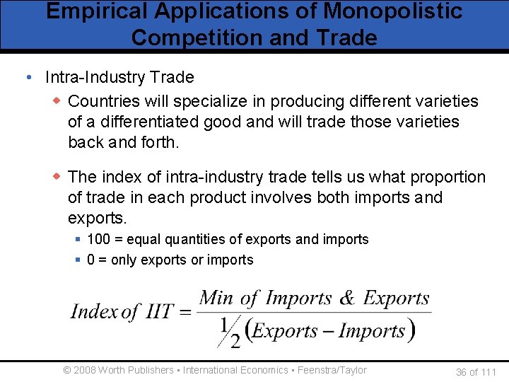
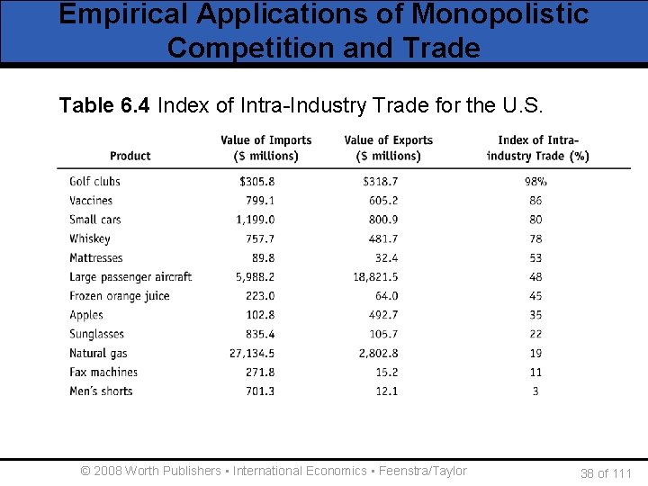
Empirical Applications of Monopolistic Competition and Trade • Intra-Industry Trade w Countries will specialize in producing different varieties of a differentiated good and will trade those varieties back and forth. w The index of intra-industry trade tells us what proportion of trade in each product involves both imports and exports. § 100 = equal quantities of exports and imports § 0 = only exports or imports © 2008 Worth Publishers ▪ International Economics ▪ Feenstra/Taylor 36 of 111

Empirical Applications of Monopolistic Competition and Trade • Index of Intra-Industry Trade w For the golf clubs, we can use data from Table 6. 1. w The minimum of imports and exports is $305. 8. w Using the other data, we have Index of IIT = 305. 8/[. 5(305. 8+318. 7)] = 98%. w In Table 6. 4 there are other examples of intra-industry trade in other products for the U. S. w To obtain a high index of intra-industry trade, it is necessary for the good to be differentiated and for costs to be similar in the Home and Foreign countries, leading to both imports and exports. © 2008 Worth Publishers ▪ International Economics ▪ Feenstra/Taylor 37 of 111

Empirical Applications of Monopolistic Competition and Trade Table 6. 4 Index of Intra-Industry Trade for the U. S. © 2008 Worth Publishers ▪ International Economics ▪ Feenstra/Taylor 38 of 111

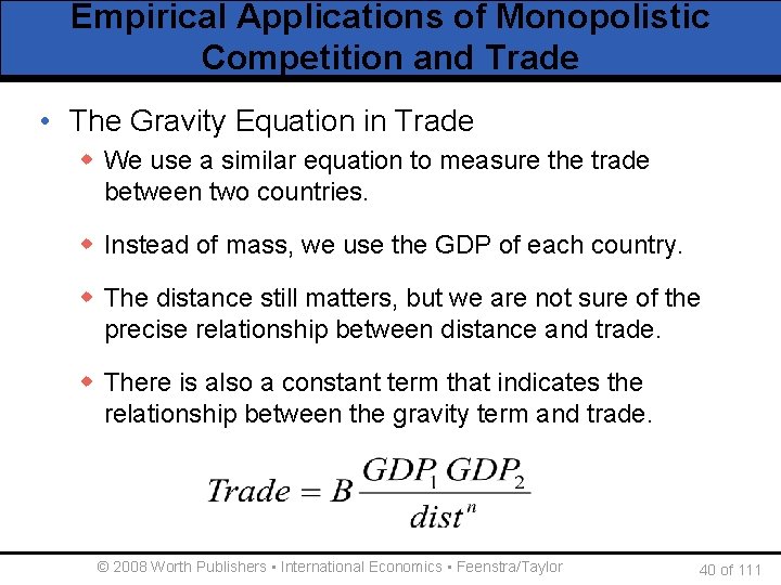
Empirical Applications of Monopolistic Competition and Trade • The Gravity Equation w To explain the value of trade, we need a different equation called the gravity equation. w Dutch economist and Nobel laureate, Jan Tinbergen was trained in physics and thought the trade between countries was similar to the force of gravity between objects. § Objects with larger mass or those that are close together have greater gravitational pull between them. w The force of gravity between these two masses is: Fg = G[M 1 M 2/d 2] § G is the constant that tells the magnitude of the relationship. § M 1 and M 2 are the two objects’ masses. © 2008 Worth Publishers ▪ International Economics ▪ Feenstra/Taylor 39 of 111

Empirical Applications of Monopolistic Competition and Trade • The Gravity Equation in Trade w We use a similar equation to measure the trade between two countries. w Instead of mass, we use the GDP of each country. w The distance still matters, but we are not sure of the precise relationship between distance and trade. w There is also a constant term that indicates the relationship between the gravity term and trade. © 2008 Worth Publishers ▪ International Economics ▪ Feenstra/Taylor 40 of 111

Empirical Applications of Monopolistic Competition and Trade • The Gravity Equation in Trade w The constant term can also be interpreted as summarizing the effects of all factors, other than distance and size, that influence the amount of trade between two countries. w The effect of size is an implication of the monopolistic competition model we studied in this chapter. § Larger countries export more because they produce more product varieties, and import more because their demand is higher. © 2008 Worth Publishers ▪ International Economics ▪ Feenstra/Taylor 41 of 111

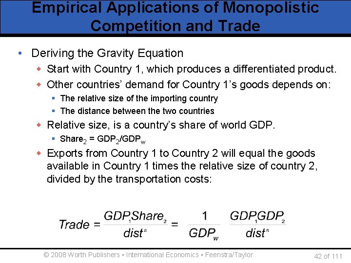
Empirical Applications of Monopolistic Competition and Trade • Deriving the Gravity Equation w Start with Country 1, which produces a differentiated product. w Other countries’ demand for Country 1’s goods depends on: § The relative size of the importing country § The distance between the two countries w Relative size, is a country’s share of world GDP. § Share 2 = GDP 2/GDPw w Exports from Country 1 to Country 2 will equal the goods available in Country 1 times the relative size of country 2, divided by the transportation costs: © 2008 Worth Publishers ▪ International Economics ▪ Feenstra/Taylor 42 of 111

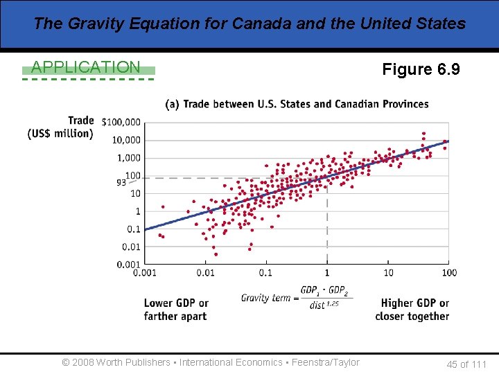
The Gravity Equation for Canada and the United States APPLICATION • Figure 6. 9 shows data collected on the value of trade between Canadian provinces and the U. S. states in 1993. • An exponent of 1. 25 is used on the distance variable based on other research studies. • The horizontal axis is the log of the gravity equation The higher the value means either a large GDP for the trading province and state or a smaller distance between them • The vertical axis shows the 1993 value of exports between a Canadian province and U. S. state or vice versa, again in logarithms. © 2008 Worth Publishers ▪ International Economics ▪ Feenstra/Taylor 43 of 111

The Gravity Equation for Canada and the United States APPLICATION • Each of the points in panel A represents the trade flow and gravity term between one state and one province. • We can see that a pair with a high gravity term also has more trade. w This supports the gravity equation theory. • We can also estimate a best fit line through the data points which gives a constant term of 93. w When the gravity term equals 1, then the predicted amount of trade between that state and province is $93 million. © 2008 Worth Publishers ▪ International Economics ▪ Feenstra/Taylor 44 of 111

The Gravity Equation for Canada and the United States APPLICATION © 2008 Worth Publishers ▪ International Economics ▪ Feenstra/Taylor Figure 6. 9 45 of 111

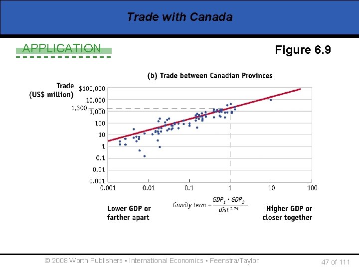
Trade with Canada APPLICATION • The gravity equation should also work well at predicting trade within a country, or intra-national trade. • Panel B of figure 6. 9 graphs the value of exports and the gravity term between any two Canadian provinces. • There is a strong positive relationship between the gravity term between two provinces and their trade. • The best fit line gives a constant term of 1300. w When gravity term is 1, the predicted amount of trade is $1. 3 billion. © 2008 Worth Publishers ▪ International Economics ▪ Feenstra/Taylor 46 of 111

Trade with Canada APPLICATION © 2008 Worth Publishers ▪ International Economics ▪ Feenstra/Taylor Figure 6. 9 47 of 111

Trade with Canada APPLICATION • Taking the ratio of the constant terms (1300/93 = 14), means on average there is 14 times more trade within Canada than occurs across the border. • The number is even higher if we consider an earlier year before the free trade agreement. w In 1988, intra-national trade within Canada was 22 times higher. • The fact that there is so much trade within Canada reflects all the barriers to trade that occur between countries. w Tariffs and Quotas w Other administrative rules and regulations w Geographic an cultural factors © 2008 Worth Publishers ▪ International Economics ▪ Feenstra/Taylor 48 of 111

Imperfect Competition with Homogeneous Products: The Case of Dumping • While product differentiation is a good assumption for many goods, it does not hold for unprocessed goods traded between firms. w Chemicals, lumber, minerals, steel, can all be treated as homogeneous. • However, in many of these goods, the markets are not perfectly competitive. w We want to assume imperfect competition here even though the goods are homogeneous. • With imperfect competition, firms can charge different prices across countries and will do so whenever it is profitable. © 2008 Worth Publishers ▪ International Economics ▪ Feenstra/Taylor 49 of 111

Imperfect Competition with Homogeneous Products: The Case of Dumping • A Model of Product Dumping w Dumping occurs when a firm sells a product abroad at a price that is either less than the price it charges in its local market, or less than its average cost to produce the product. w Under the rules of the WTO, am importing country is entitled to apply a tariff, called an antidumping duty any time a foreign firm dumps its product on a local market. w Why do firms dump at all? © 2008 Worth Publishers ▪ International Economics ▪ Feenstra/Taylor 50 of 111

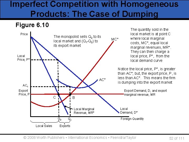
Imperfect Competition with Homogeneous Products: The Case of Dumping • Discriminating Monopoly w Assume a foreign monopolist sells both to its local market and exports to Home. w The monopolist is able to charge different prices in the two markets. § Discriminating monopoly w Firm has a monopoly at home but faces a competitive export market § Downward sloping demand curve in home market. § Horizontal demand curve in export market. w Consider the following example: © 2008 Worth Publishers ▪ International Economics ▪ Feenstra/Taylor 51 of 111

Imperfect Competition with Homogeneous Products: The Case of Dumping Figure 6. 10 Price The monopolist sells Q 2 to its local market and (Q 1 -Q 2) to its export market Local Price, P* AC 1 Export Price, P C B Local Marginal Revenue, MR* Q 2 Local Sales Q 1 MC* The sold in the Thequantity export monopoly local market profits is at point maximizes at C where marginal point local B where local costs, MC*, equal local marginal costs, MC*, marginal revenues, MR*. equal export marginal They can then revenues, MRcharge a local price, P*, from the local demand curve Notice the local price, P*, is greater than AC*; but, the export price, P, is less than AC*. This means the firm is dumping into the export market Export Demand, D, and export marginal revenue, MR Local Demand, D* Foreign Quantity Exports © 2008 Worth Publishers ▪ International Economics ▪ Feenstra/Taylor 52 of 111

Imperfect Competition with Homogeneous Products: The Case of Dumping • The Profitability of Dumping w The Foreign firm charges P* selling Q 2 in the local market. w The local price is higher than the export price. § It is dumping its product into the export market. w The average costs are lower than the local price but higher than the export price. w Since AC is above the export price, the firm is also dumping according to this cost comparison. © 2008 Worth Publishers ▪ International Economics ▪ Feenstra/Taylor 53 of 111

Imperfect Competition with Homogeneous Products: The Case of Dumping • Numerical Example of Dumping w Suppose the following data: § Fixed costs = $100; Marginal costs = $10/unit § Local price = $25; Local quantity = 10 § Export price = $15; Export quantity = 10 w Profits from the local market are: § $25(10) - $100 = $50 w Average costs for the firms are $20. w Profits in the export market are: § [$25(10) + $15(10)] - $10(20) - $100 = $100 w The export price is below AC but above MC. © 2008 Worth Publishers ▪ International Economics ▪ Feenstra/Taylor 54 of 111

Imperfect Competition with Homogeneous Products: The Case of Dumping • Reciprocal Dumping w It can happen that firms in both countries are accused of dumping in the other—this is reciprocal dumping. w For example, shortly after the U. S. ruled that Canadian greenhouse tomatoes were being dumped into the U. S. , the Canadian government investigated dumping against American fresh tomatoes. w The final ruling was that there was no harm or injury to the firms in either country, so no antidumping duties were applied. © 2008 Worth Publishers ▪ International Economics ▪ Feenstra/Taylor 55 of 111

Imperfect Competition with Homogeneous Products: The Case of Dumping • Reciprocal Dumping w How can it be profitable for both firms to charge prices for their exports that are below their local prices? w We show that, in fact, it is a common feature of imperfectly competitive markets. w Rather than selling additional units in the local market and depressing its own price, a firm can enter the export market. w It then depresses the price of firms abroad by increasing quantity. w Since both firms have this incentive, equilibrium will have both firms selling abroad. © 2008 Worth Publishers ▪ International Economics ▪ Feenstra/Taylor 56 of 111

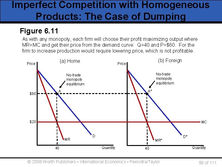
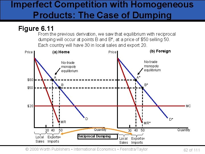
Imperfect Competition with Homogeneous Products: The Case of Dumping • Numerical Example of Reciprocal Dumping w Assume Home and Foreign have identical demand curves: P = 100 – Q w Remember, marginal revenue, MR = P – ΔP*Q w The price drops $1 for even extra unit sold, so ΔP=1 and MR = P-Q, this gives: § MR = P – Q = (100 – Q) – Q = 100 – 2 Q w Home and Foreign have identical MC = $20/unit. w Without trade, we get the monopoly equilibrium § Q = 40 and P = $60 © 2008 Worth Publishers ▪ International Economics ▪ Feenstra/Taylor 57 of 111

Imperfect Competition with Homogeneous Products: The Case of Dumping Figure 6. 11 As with any monopoly, each firm will choose their profit maximizing output where MR=MC and get their price from the demand curve: Q=40 and P=$60. For the firm to increase production would require lowering price, which is not profitable. (a) Home Price (b) Foreign Price No-trade monopoly equilibrium $60 A A* $20 MC MR 40 D MR* Quantity 40 © 2008 Worth Publishers ▪ International Economics ▪ Feenstra/Taylor D* Quantity 58 of 111

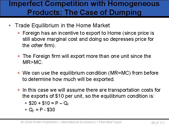
Imperfect Competition with Homogeneous Products: The Case of Dumping • Trade Equilibrium in the Home Market w Foreign has an incentive to export to Home (since price is still above marginal cost and doing so depresses price for the other firm). w The Foreign firm will export more than one unit since the MR>MC. w We can use the equilibrium condition (MR=MC) from before to determine how much will be exported. w In this case we will assume there are transportation costs for the exports of $10 per unit, so the equilibrium condition is: § $20 + $10 = P – QF § QF = P - $30 © 2008 Worth Publishers ▪ International Economics ▪ Feenstra/Taylor 59 of 111

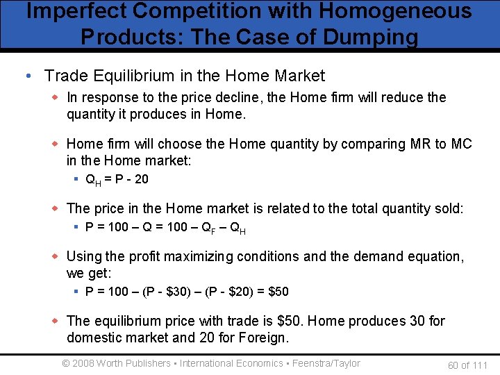
Imperfect Competition with Homogeneous Products: The Case of Dumping • Trade Equilibrium in the Home Market w In response to the price decline, the Home firm will reduce the quantity it produces in Home. w Home firm will choose the Home quantity by comparing MR to MC in the Home market: § QH = P - 20 w The price in the Home market is related to the total quantity sold: § P = 100 – QF – QH w Using the profit maximizing conditions and the demand equation, we get: § P = 100 – (P - $30) – (P - $20) = $50 w The equilibrium price with trade is $50. Home produces 30 for domestic market and 20 for Foreign. © 2008 Worth Publishers ▪ International Economics ▪ Feenstra/Taylor 60 of 111

Imperfect Competition with Homogeneous Products: The Case of Dumping • Two-way Trade w Since the Foreign firm has an incentive to enter the Home market and both firms are the same, the Home firm has the same incentive in the Foreign market. w Foreign price with trade will also be $50 with Foreign producing 30 units for its own market and importing 20 units from Home. § B and B* in figure 6. 11 w Notice that as each firm sells in the other market, prices fall in both market. Firms are engaged in “reciprocal dumping” © 2008 Worth Publishers ▪ International Economics ▪ Feenstra/Taylor 61 of 111

Imperfect Competition with Homogeneous Products: The Case of Dumping Figure 6. 11 From theequal previous derivation, sawand that. Foreign equilibrium reciprocal Exports imports for bothwe Home fromwith each dumping will occur Dumping at points B and B*, at a price of $50 selling 50. other – Reciprocal Each country will have 30 in local sales and export 20. (a) Home Price (b) Foreign Price No-trade monopoly equilibrium A $60 A* B $50 B* $20 MC MR 30 40 Local Sales 50 Exports= Imports D MR* Quantity Reciprocal Dumping 30 40 50 Local Sales D* Quantity Exports= Imports © 2008 Worth Publishers ▪ International Economics ▪ Feenstra/Taylor 62 of 111

Imperfect Competition with Homogeneous Products: The Case of Dumping • Measurement of Dumping w In trade disputes over dumping, the government in each country compares the price that a Foreign firm earns in the country’s market, net of transportation costs, to the price the Foreign firm earns in its local market. w In our example, Foreign exports at $50 with $10 in transportation costs: net $40. w Since the price in local market is $50, Foreign is dumping in the Home market. w Similarly, Home is dumping into the Foreign market. w Reciprocal dumping is occurring. © 2008 Worth Publishers ▪ International Economics ▪ Feenstra/Taylor 63 of 111

Imperfect Competition with Homogeneous Products: The Case of Dumping • Measurement of Dumping w This example has allowed us to illustrate the incentives for firms to enter markets abroad. w For the first units sold to the export market, the MR for the exporting firm will always be higher than the MR of the local firm abroad. § The exporting firm does not lose as much revenue from existing sales by selling additional units in the export market. w The Foreign firm has an incentive to enter the Home market and the Home firm has an incentive to enter the Foreign market. w We should not be surprised to see two-way trade even with homogeneous products. © 2008 Worth Publishers ▪ International Economics ▪ Feenstra/Taylor 64 of 111