6 Dynamic Programming II sequence alignment Hirschbergs algorithm

6. Dynamic Programming II ‣ sequence alignment ‣ Hirschberg's algorithm ‣ Bellman-Ford algorithm ‣ distance vector protocols ‣ negative cycles in a digraph Lecture slides by Kevin Wayne Copyright © 2005 Pearson-Addison Wesley Copyright © 2013 Kevin Wayne http: //www. cs. princeton. edu/~wayne/kleinberg-tardos Last updated on Oct 5, 2013 9: 39 PM

6. Dynamic Programming II ‣ sequence alignment ‣ Hirschberg's algorithm ‣ Bellman-Ford algorithm ‣ distance vector protocols ‣ negative cycles in a digraph Section 6. 6

String similarity Q. How similar are two strings? Ex. ocurrance and occurrence. o c u r r a n c e – o c – u r r a n c e o c c u r r e n c e 6 mismatches, 1 gap 1 mismatch, 1 gap o c – u r r – a n c e o c c u r r e – n c e 0 mismatches, 3 gaps 3

Edit distance. [Levenshtein 1966, Needleman-Wunsch 1970] ・Gap penalty δ; mismatch penalty αpq. ・Cost = sum of gap and mismatch penalties. C T – G A C C T A C G C T G G A C G A A C G cost = δ + αCG + αTA Applications. Unix diff, speech recognition, computational biology, . . . 4

Sequence alignment Goal. Given two strings x 1 x 2. . . xm and y 1 y 2. . . yn find min cost alignment. Def. An alignment M is a set of ordered pairs xi – yj such that each item occurs in at most one pair and no crossings. xi – yj and xi' – yj' cross if i < i ', but j > j ' Def. The cost of an alignment M is: x 1 x 2 x 3 x 4 x 5 x 6 C T A C C – G – T A C A T G y 1 y 2 y 3 y 4 y 5 y 6 an alignment of CTACCG and TACATG: M = { x 2–y 1, x 3–y 2, x 4–y 3, x 5–y 4, x 6–y 6 } 5

Sequence alignment: problem structure Def. OPT(i, j) = min cost of aligning prefix strings x 1 x 2. . . xi and y 1 y 2. . . yj. Case 1. OPT matches xi – yj. Pay mismatch for xi – yj + min cost of aligning x 1 x 2. . . xi– 1 and y 1 y 2. . . yj– 1. Case 2 a. OPT leaves xi unmatched. Pay gap for xi + min cost of aligning x 1 x 2. . . xi– 1 and y 1 y 2. . . yj. Case 2 b. OPT leaves yj unmatched. optimal substructure property (proof via exchange argument) Pay gap for yj + min cost of aligning x 1 x 2. . . xi and y 1 y 2. . . yj– 1. 6

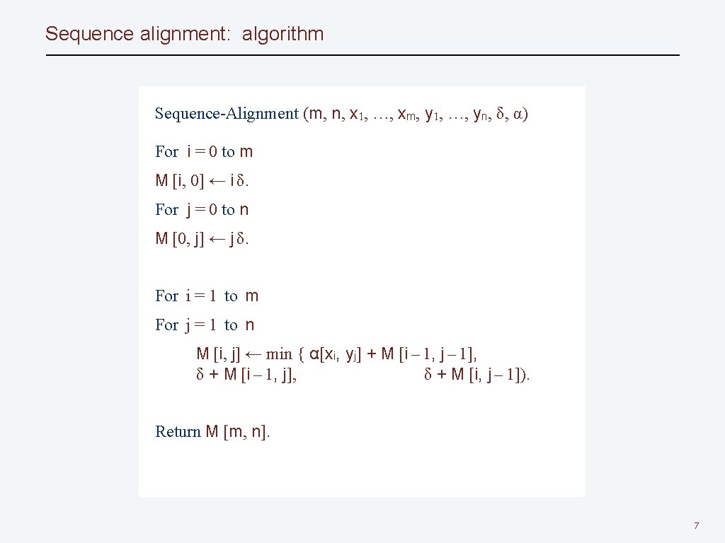
Sequence alignment: analysis Theorem. The dynamic programming algorithm computes the edit distance (and optimal alignment) of two strings of length m and n in Θ(mn) time and Θ(mn) space. Pf. ・Algorithm computes edit distance. ・Can trace back to extract optimal alignment itself. ▪ Q. Can we avoid using quadratic space? A. Easy to compute optimal value in O(mn) time and O(m + n) space. ・Compute OPT(i, • ) from OPT(i – 1, • ). ・But, no longer easy to recover optimal alignment itself. 8

6. Dynamic Programming II ‣ sequence alignment ‣ Hirschberg's algorithm ‣ Bellman-Ford algorithm ‣ distance vector protocols ‣ negative cycles in a digraph Section 6. 7

Sequence alignment in linear space Theorem. There exist an algorithm to find an optimal alignment in O(mn) time and O(m + n) space. ・Clever combination of divide-and-conquer and dynamic programming. ・Inspired by idea of Savitch from complexity theory. 10

Hirschberg's algorithm ε ε y 1 y 2 y 3 y 4 y 5 y 6 0 -0 x 1 δ i-j x 2 δ x 3 m-n 11

Hirschberg's algorithm ▪ δ i-j δ 12

Hirschberg's algorithm j ε ε y 1 y 2 y 3 y 4 y 5 y 6 0 -0 x 1 x 2 x 3 i-j m-n 13

Hirschberg's algorithm ε ε y 1 y 2 y 3 y 4 y 5 y 6 0 -0 i-j x 1 δ δ x 2 x 3 m-n 14

Hirschberg's algorithm j ε ε x 1 y 2 y 3 y 4 y 5 y 6 0 -0 i-j x 2 x 3 m-n 15

Hirschberg's algorithm Observation 1. The cost of the shortest path that uses (i, j) is f (i, j) + g(i, j). ε ε x 1 y 2 y 3 y 4 y 5 y 6 0 -0 i-j x 2 x 3 m-n 16

Hirschberg's algorithm n/2 ε ε x 1 y 2 y 3 y 4 y 5 y 6 0 -0 i-j q x 2 x 3 m-n 17

Hirschberg's algorithm n/2 ε ε x 1 y 2 y 3 y 4 y 5 y 6 0 -0 i-j q x 2 x 3 m-n 18

Hirschberg's algorithm: running time analysis warmup Theorem. Let T(m, n) = max running time of Hirschberg's algorithm on strings of length at most m and n. Then, T(m, n) = O(m n log n). Pf. T(m, n) ≤ 2 T(m, n / 2) + O(m n) ⇒ T(m, n) = O(m log n). Remark. Analysis is not tight because two subproblems are of size (q, n/2) and (m – q, n / 2). In next slide, we save log n factor. 19

Hirschberg's algorithm: running time analysis Theorem. Let T(m, n) = max running time of Hirschberg's algorithm on strings of length at most m and n. Then, T(m, n) = O(m n). Pf. [ by induction on n ] ・O(m n) time to compute f ( • , n / 2) and g ( • , n / 2) and find index q. ・T(q, n / 2) + T(m – q, n / 2) time for two recursive calls. ・Choose constant c so that: T(m, 2) ≤ c m ・Claim. T(m, n) ≤ 2 c m n. ・Base cases: m = 2 or n = 2. ・Inductive hypothesis: T(m, n) T(2, n) ≤ cn T(m, n) ≤ c m n + T(q, n / 2) + T(m – q, n / 2) ≤ 2 c m n for all (m', n') with m' + n' < m + n. ≤ T(q, n / 2) + T(m – q, n / 2) + c m n ≤ 2 c q n / 2 + 2 c (m – q) n / 2 + c m n = cq n + cmn – cqn + cmn = 2 cmn ▪ 20

6. Dynamic Programming II ‣ sequence alignment ‣ Hirschberg's algorithm ‣ Bellman-Ford ‣ distance vector protocols ‣ negative cycles in a digraph Section 6. 8

Shortest paths Shortest path problem. Given a digraph G = (V, E), with arbitrary edge weights or costs cvw, find cheapest path from node s to node t. 3 1 5 source s 0 8 9 1 2 7 7 -1 5 3 4 4 3 5 9 2 1 11 5 13 10 6 destination t cost of path = 9 - 3 + 11 = 18 22

Shortest paths: failed attempts Dijkstra. Can fail if negative edge weights. s 2 u 3 1 8 v w Reweighting. Adding a constant to every edge weight can fail. u 5 5 2 2 s t 6 7 3 v 0 3 3 w 23

Negative cycles Def. A negative cycle is a directed cycle such that the sum of its edge weights is negative. 5 3 -3 4 4 a negative cycle W : 24

Shortest paths and negative cycles Lemma 1. If some path from v to t contains a negative cycle, then there does not exist a cheapest path from v to t. Pf. If there exists such a cycle W, then can build a v↝t path of arbitrarily negative weight by detouring around cycle as many times as desired. ▪ v t W c(W) < 0 25

Shortest paths and negative cycles Lemma 2. If G has no negative cycles, then there exists a cheapest path from v to t that is simple (and has ≤ n – 1 edges). Pf. ・Consider a cheapest v↝t path P that uses the fewest number of edges. ・If P contains a cycle W, can remove portion of P corresponding to W without increasing the cost. ▪ v t W c(W) ≥ 0 26

Shortest path and negative cycle problems Shortest path problem. Given a digraph G = (V, E) with edge weights cvw and no negative cycles, find cheapest v↝t path for each node v. Negative cycle problem. Given a digraph G = (V, E) with edge weights cvw, find a negative cycle (if one exists). 5 1 4 2 3 5 t shortest-paths tree 3 -3 4 4 negative cycle 27

Shortest paths: dynamic programming Def. OPT(i, v) = cost of shortest v↝t path that uses ≤ i edges. ・Case 1: Cheapest v↝t path uses ≤ i – 1 edges. - OPT(i, v) = OPT(i – 1, v) ・Case 2: Cheapest v↝t path uses exactly i edges. optimal substructure property (proof via exchange argument) - if (v, w) is first edge, then OPT uses (v, w), and then selects best w↝t path using ≤ i – 1 edges ∞ Observation. If no negative cycles, OPT(n – 1, v) = cost of cheapest v↝t path. Pf. By Lemma 2, cheapest v↝t path is simple. ▪ 28

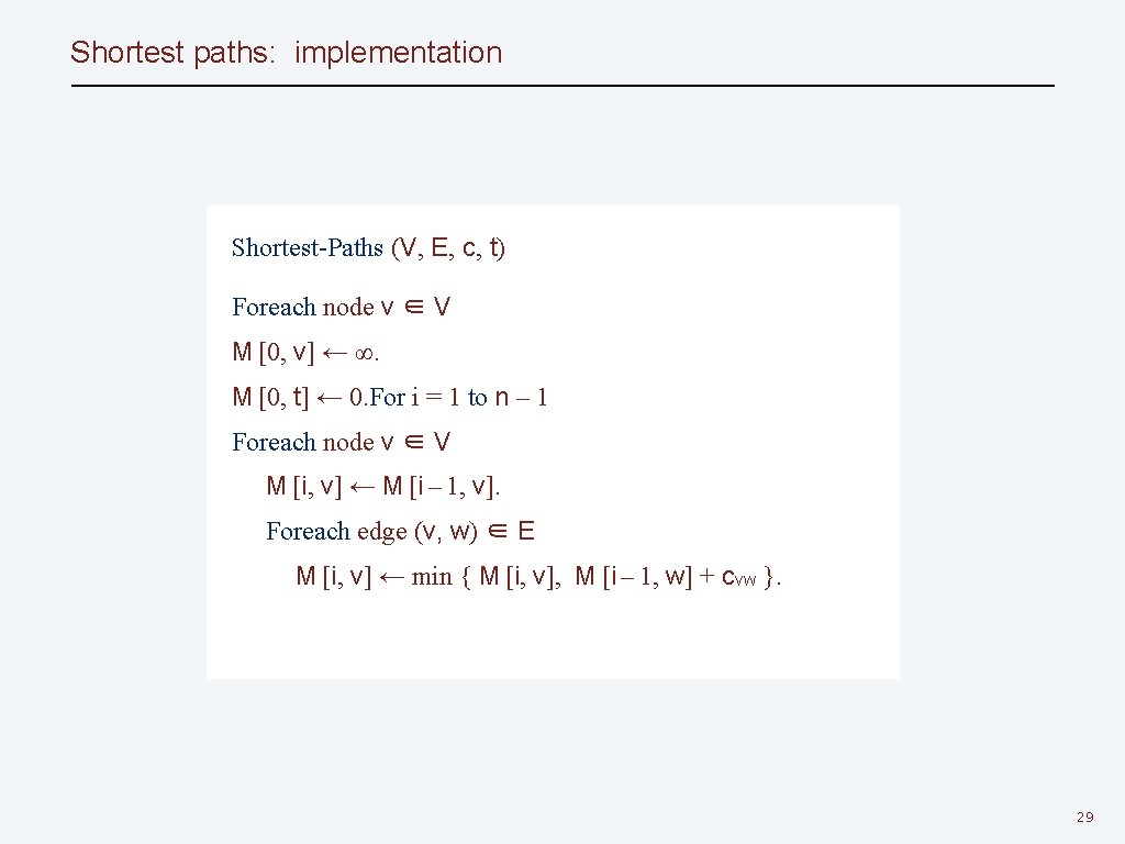
Shortest paths: implementation Theorem 1. Given a digraph G = (V, E) with no negative cycles, the dynamic programming algorithm computes the cost of the cheapest v↝t path for each node v in Θ(mn) time and Θ(n 2) space. Pf. ・Table requires Θ(n 2) space. ・Each iteration i takes Θ(m) time since we examine each edge once. ▪ Finding the shortest paths. ・Approach 1: Maintain a successor(i, v) that points to next node on cheapest v↝t path using at most i edges. ・Approach 2: Compute optimal costs M[i, v] and consider only edges with M[i, v] = M[i – 1, w] + cvw. 30

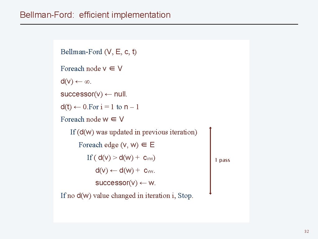
Shortest paths: practical improvements Space optimization. Maintain two 1 d arrays (instead of 2 d array). ・d(v) = cost of cheapest v↝t path that we have found so far. ・successor(v) = next node on a v↝t path. Performance optimization. If d(w) was not updated in iteration i – 1, then no reason to consider edges entering w in iteration i. 31

Bellman-Ford: analysis Claim. After the ith pass of Bellman-Ford, d(v) equals the cost of the cheapest v↝t path using at most i edges. Counterexample. Claim is false! d(v) = 3 v d(t) = 0 d(w) = 2 1 w 2 t 4 if nodes w considered before node v, then d(v) = 3 after 1 pass 33

Bellman-Ford: analysis Lemma 3. Throughout Bellman-Ford algorithm, d(v) is the cost of some v↝t path; after the ith pass, d(v) is no larger than the cost of the cheapest v↝t path using ≤ i edges. Pf. [by induction on i] ・Assume true after ith pass. ・Let P be any v↝t path with i + 1 edges. ・Let (v, w) be first edge on path and let P' be subpath from w to t. ・By inductive hypothesis, d(w) ≤ c(P') since P' is a w↝t path with i edges. ・After considering v in pass i+1: d(v) ≤ c + d(w) vw ≤ cvw + c(P') = c(P) ▪ Theorem 2. Given a digraph with no negative cycles, Bellman-Ford computes the costs of the cheapest v↝t paths in O(mn) time and Θ(n) extra space. Pf. Lemmas 2 + 3. ▪ can be substantially faster in practice 34

Bellman-Ford: analysis consider nodes in order: t, 1, 2, 3 s(2) = 1 d(2) = 20 2 1 0 s(1) = t d(1) = 10 1 1 s(3) = t d(3) = 1 1 0 d(t) = 0 t 1 3 35

Bellman-Ford: analysis consider nodes in order: t, 1, 2, 3 s(2) = 1 d(2) = 20 2 1 0 s(1) = 3 d(1) = 2 1 1 s(3) = t d(3) = 1 1 0 d(t) = 0 t 1 3 36

Bellman-Ford: analysis consider nodes in order: t, 1, 2, 3, 4 d(2) = 8 d(3) = 10 3 2 2 9 4 d(4) = 11 t 3 1 8 d(t) = 0 5 1 d(1) = 5 37

Bellman-Ford: analysis consider nodes in order: t, 1, 2, 3, 4 d(2) = 8 d(3) = 10 3 2 2 9 4 d(4) = 11 t 3 1 8 d(t) = 0 5 1 d(1) = 3 38

Bellman-Ford: finding the shortest path Lemma 4. If the successor graph contains a directed cycle W, then W is a negative cycle. Pf. ・If successor(v) = w, we must have d(v) ≥ d(w) + cvw. (LHS and RHS are equal when successor(v) is set; d(w) can only decrease; d(v) decreases only when successor(v) is reset) ‣ Let v → … → v be the nodes along the cycle W. ・Assume that (v , v ) is the last edge added to the successor graph. ・Just prior to that: d(v ) ≥ d(v ) + c(v , v ) 1 2 k k 1 1 ‣ 2 d(v 3) 1 2 d(v 2) ≥ + c(v 2, v 3) ⋮ ⋮ d(vk– 1) ≥ d(vk) + c(vk– 1, vk) d(vk) > d(v 1) + c(vk, v 1) ⋮ holds with strict inequality since we are updating d(vk) Adding inequalities yields c(v 1, v 2) + c(v 2, v 3) + … + c(vk– 1, vk) + c(vk, v 1) < 0. ▪ W is a negative cycle 39

Bellman-Ford: finding the shortest path Theorem 3. Given a digraph with no negative cycles, Bellman-Ford finds the cheapest s↝t paths in O(mn) time and Θ(n) extra space. Pf. ・The successor graph cannot have a negative cycle. [Lemma 4] ・Thus, following the successor pointers from s yields a directed path to t. ・Let s = v 1 → v 2 → … → vk = t be the nodes along this path P. ・Upon termination, if successor(v) = w, we must have d(v) = d(w) + cvw. (LHS and RHS are equal when successor(v) is set; d(·) did not change) ・Thus, ・ d(v 1) = d(v 2) + c(v 1, v 2) d(v 2) = d(v 3) + c(v 2, v 3) ⋮ ⋮ d(vk– 1) = ⋮ d(vk) since algorithm terminated + c(vk– 1, vk) Adding equations yields d(s) = d(t) + c(v 1, v 2) + c(v 2, v 3) + … + c(vk– 1, vk). ▪ min cost of any s↝t path (Theorem 2) 0 cost of path P 40

6. Dynamic Programming II ‣ sequence alignment ‣ Hirschberg's algorithm ‣ Bellman-Ford ‣ distance vector protocols ‣ negative cycles in a digraph Section 6. 9

Distance vector protocols Communication network. ・Node ≈ router. ・Edge ≈ direct communication link. ・Cost of edge ≈ delay on link. naturally nonnegative, but Bellman-Ford used anyway! Dijkstra's algorithm. Requires global information of network. Bellman-Ford. Uses only local knowledge of neighboring nodes. Synchronization. We don't expect routers to run in lockstep. The order in which each foreach loop executes in not important. Moreover, algorithm still converges even if updates are asynchronous. 42

Distance vector protocols. [ "routing by rumor" ] ・Each router maintains a vector of shortest path lengths to every other node (distances) and the first hop on each path (directions). ・Algorithm: each router performs n separate computations, one for each potential destination node. Ex. RIP, Xerox XNS RIP, Novell's IPX RIP, Cisco's IGRP, DEC's DNA Phase IV, Apple. Talk's RTMP. Caveat. Edge costs may change during algorithm (or fail completely). 1 s d(s) = 2 1 deleted v d(v) = 1 "counting to infinity" 1 t d(t) = 0 43

Path vector protocols Link state routing. not just the distance and first hop ・Each router also stores the entire path. ・Based on Dijkstra's algorithm. ・Avoids "counting-to-infinity" problem and related difficulties. ・Requires significantly more storage. Ex. Border Gateway Protocol (BGP), Open Shortest Path First (OSPF). 44

6. Dynamic Programming II ‣ sequence alignment ‣ Hirschberg's algorithm ‣ Bellman-Ford ‣ distance vector protocol ‣ negative cycles in a digraph Section 6. 10

Detecting negative cycles Negative cycle detection problem. Given a digraph G = (V, E), with edge weights cvw, find a negative cycle (if one exists). 5 -3 2 4 6 4 3 3 4 46

Detecting negative cycles: application Currency conversion. Given n currencies and exchange rates between pairs of currencies, is there an arbitrage opportunity? Remark. Fastest algorithm very valuable! 47

Detecting negative cycles v t W c(W) < 0 48

Detecting negative cycles Theorem 4. Can find a negative cycle in Θ(mn) time and Θ(n 2) space. Pf. ・Add new node t and connect all nodes to t with 0 -cost edge. ・G has a negative cycle iff G' has a negative cycle than can reach t. ・If OPT(n, v) = OPT(n – 1, v) for all nodes v, then no negative cycles. ・If not, then extract directed cycle from path from v to t. (cycle cannot contain t since no edges leave t) ▪ 5 -3 2 4 6 4 3 G' 3 t 4 49

Detecting negative cycles Theorem 5. Can find a negative cycle in O(mn) time and O(n) extra space. Pf. ・Run Bellman-Ford for n passes (instead of n – 1) on modified digraph. ・If no d(v) values updated in pass n, then no negative cycles. ・Otherwise, suppose d(s) updated in pass n. ・Define pass(v) = last pass in which d(v) was updated. ・Observe pass(s) = n and pass(successor(v)) ≥ pass(v) – 1 for each v. ・Following successor pointers, we must eventually repeat a node. ・Lemma 4 ⇒ this cycle is a negative cycle. ▪ Remark. See p. 304 for improved version and early termination rule. (Tarjan's subtree disassembly trick) 50