6 1 Inference for a Single Proportion p

6. 1 Inference for a Single Proportion p Statistical confidence p Confidence intervals p How confidence intervals behave

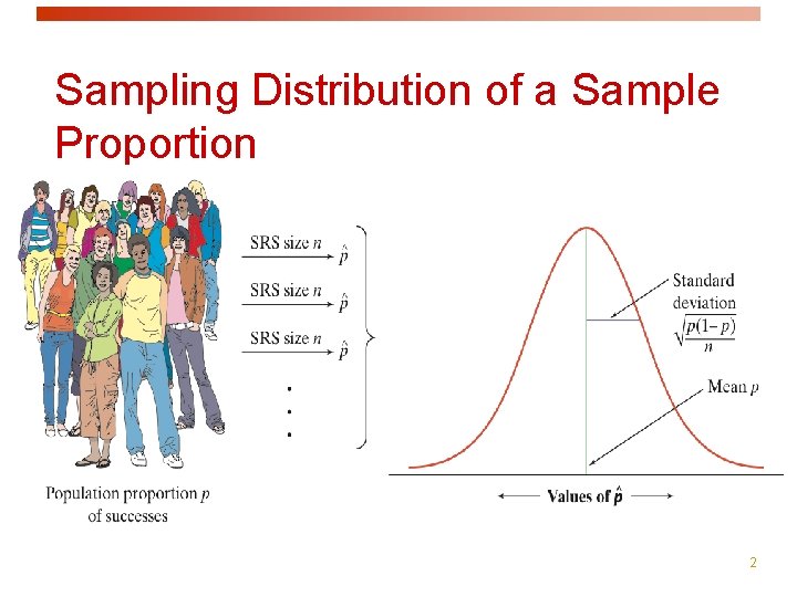
Sampling Distribution of a Sample Proportion As n increases, the sampling distribution becomes approximately Normal. 2

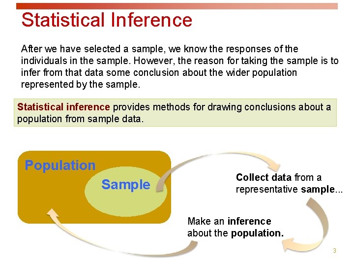
Statistical Inference After we have selected a sample, we know the responses of the individuals in the sample. However, the reason for taking the sample is to infer from that data some conclusion about the wider population represented by the sample. Statistical inference provides methods for drawing conclusions about a population from sample data. Population Sample Collect data from a representative sample. . . Make an inference about the population. 3

p p p Methods for drawing conclusions about a population from sample data are called statistical inference So we’ll use data to make these inferences; i. e. , draw conclusions about populations from data in our samples or from our experiments We'll consider two types of inference: p Confidence interval estimation p Tests of significance In both of these cases, we'll consider our data as either being a random sample from a population or as data from a randomized experiment Start with estimation… there are two situations we'll consider p estimating the mean m of a population of measurements p estimating the proportion p of Ss in a population of Ss and Fs

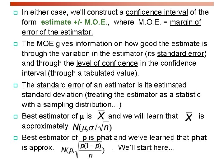
p In either case, we'll construct a confidence interval of the form estimate +/- M. O. E. , where M. O. E. = margin of error of the estimator. p The MOE gives information on how good the estimate is through the variation in the estimator (its standard error) and through the level of confidence in the confidence interval (through a tabulated value). p The standard error of an estimator is its estimated standard deviation (treating the estimator as a statistic with a sampling distribution…) p p Best estimator of m is approximately and we will learn that is Best estimator of p is phat and we’ve learned that phat is approx. . We’ll start here…

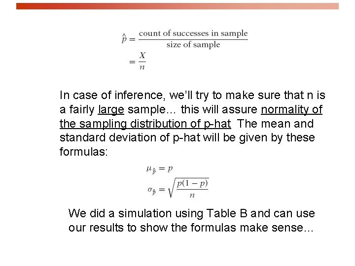
In case of inference, we’ll try to make sure that n is a fairly large sample… this will assure normality of the sampling distribution of p-hat The mean and standard deviation of p-hat will be given by these formulas: We did a simulation using Table B and can use our results to show the formulas make sense…

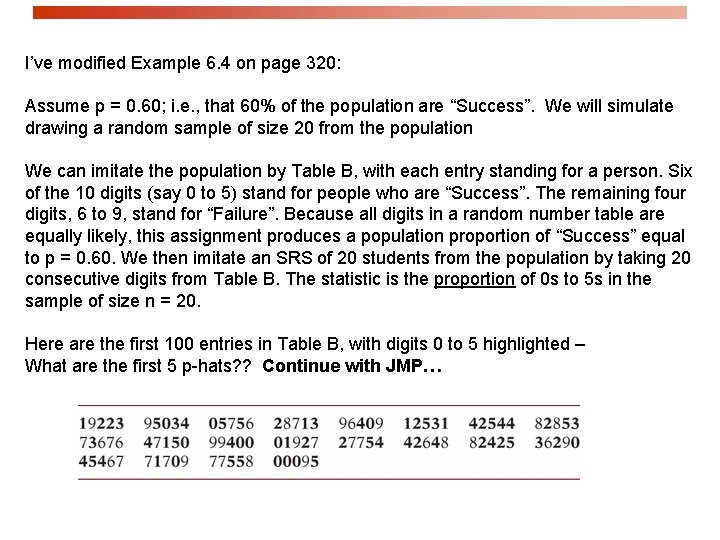
I’ve modified Example 6. 4 on page 320: Assume p = 0. 60; i. e. , that 60% of the population are “Success”. We will simulate drawing a random sample of size 20 from the population We can imitate the population by Table B, with each entry standing for a person. Six of the 10 digits (say 0 to 5) stand for people who are “Success”. The remaining four digits, 6 to 9, stand for “Failure”. Because all digits in a random number table are equally likely, this assignment produces a population proportion of “Success” equal to p = 0. 60. We then imitate an SRS of 20 students from the population by taking 20 consecutive digits from Table B. The statistic is the proportion of 0 s to 5 s in the sample of size n = 20. Here are the first 100 entries in Table B, with digits 0 to 5 highlighted – What are the first 5 p-hats? ? Continue with JMP…

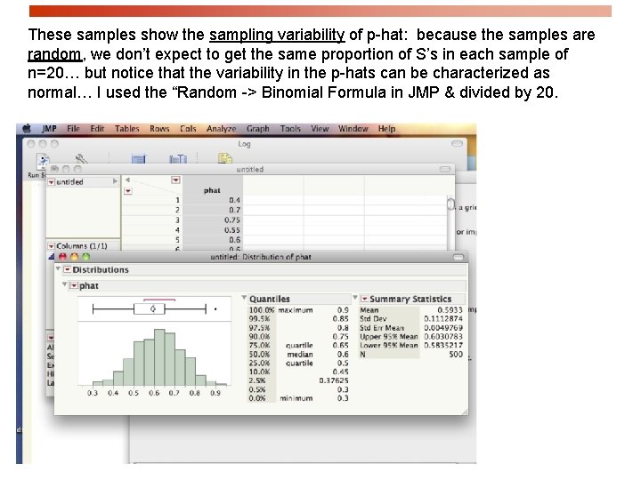
These samples show the sampling variability of p-hat: because the samples are random, we don’t expect to get the same proportion of S’s in each sample of n=20… but notice that the variability in the p-hats can be characterized as normal… I used the “Random -> Binomial Formula in JMP & divided by 20.

Sampling Distribution of a Sample Proportion As n increases, the sampling distribution becomes approximately Normal. 9

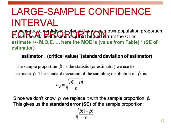
LARGE-SAMPLE CONFIDENCE INTERVAL To construct a confidence interval for an unknown population proportion FOR p we’ll use A our PROPORTION best estimator p-hat and construct the CI as estimate +/- M. O. E. … here the MOE is (value from Table) * (SE of estimator) 10

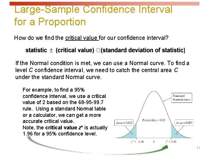
Large-Sample Confidence Interval for a Proportion How do we find the critical value for our confidence interval? If the Normal condition is met, we can use a Normal curve. To find a level C confidence interval, we need to catch the central area C under the standard Normal curve. For example, to find a 95% confidence interval, we use a critical value of 2 based on the 68 -95 -99. 7 rule. Using a standard Normal table or a calculator, we can get a more accurate critical value. Note, the critical value z* is actually 1. 96 for a 95% confidence level. 11

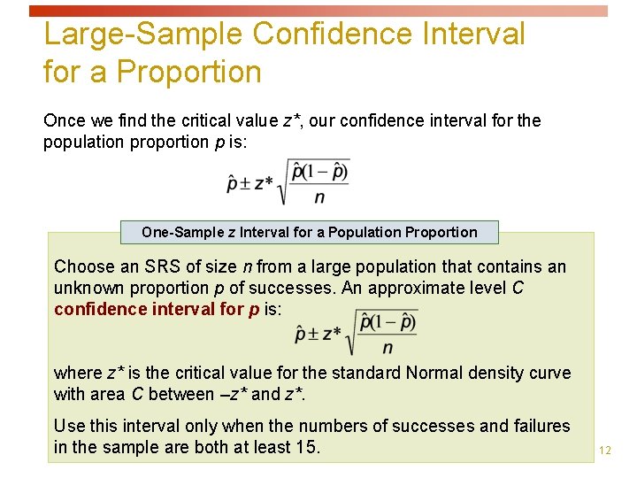
Large-Sample Confidence Interval for a Proportion Once we find the critical value z*, our confidence interval for the population proportion p is: One-Sample z Interval for a Population Proportion Choose an SRS of size n from a large population that contains an unknown proportion p of successes. An approximate level C confidence interval for p is: where z* is the critical value for the standard Normal density curve with area C between –z* and z*. Use this interval only when the numbers of successes and failures in the sample are both at least 15. 12

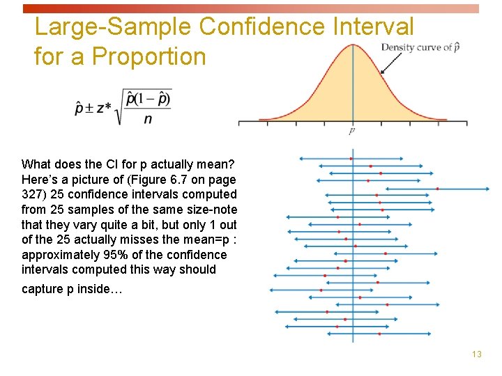
Large-Sample Confidence Interval for a Proportion What does the CI for p actually mean? Here’s a picture of (Figure 6. 7 on page 327) 25 confidence intervals computed from 25 samples of the same size-note that they vary quite a bit, but only 1 out of the 25 actually misses the mean=p : approximately 95% of the confidence intervals computed this way should capture p inside… 13

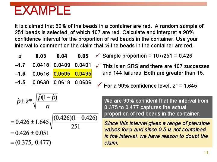
EXAMPLE It is claimed that 50% of the beads in a container are red. A random sample of 251 beads is selected, of which 107 are red. Calculate and interpret a 90% confidence interval for the proportion of red beads in the container. Use your interval to comment on the claim that ½ the beads in the container are red. z – 1. 7 0. 03 0. 04 0. 05 ü Sample proportion = 107/251 = 0. 426 – 1. 6 0. 0418 0. 0409 0. 0401 ü This is an SRS and there are 107 successes and 144 failures. Both are greater than 15. 0. 0516 0. 0505 0. 0495 – 1. 5 0. 0630 0. 0618 0. 0606 ü For a 90% confidence level, z* = 1. 645 We are 90% confident that the interval from 0. 375 to 0. 477 captures the actual proportion of red beads in the container. Since this interval gives a range of plausible values for p and since 0. 5 is not contained in the interval, we have reason to doubt the claim. 14

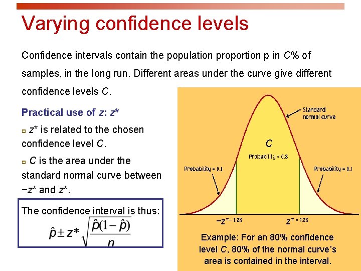
Varying confidence levels Confidence intervals contain the population proportion p in C% of samples, in the long run. Different areas under the curve give different confidence levels C. Practical use of z: z* z* is related to the chosen confidence level C. p C C is the area under the standard normal curve between −z* and z*. p The confidence interval is thus: −z* z* Example: For an 80% confidence level C, 80% of the normal curve’s area is contained in the interval.

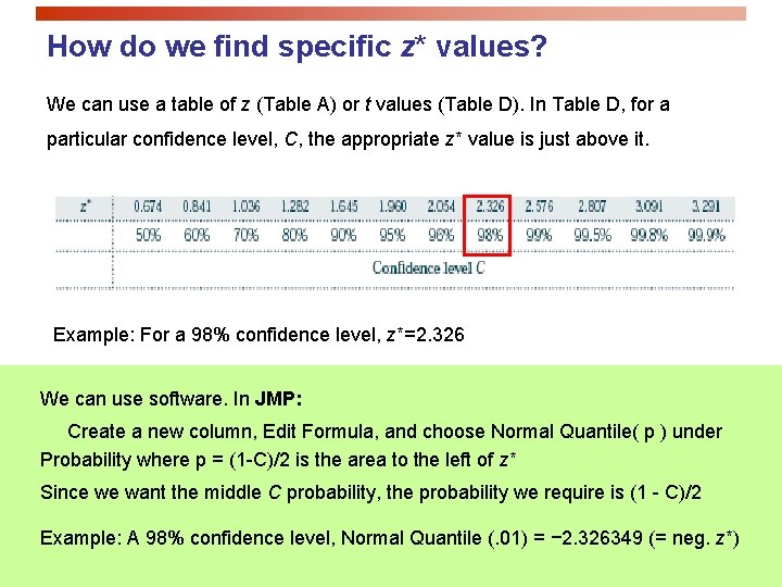
How do we find specific z* values? We can use a table of z (Table A) or t values (Table D). In Table D, for a particular confidence level, C, the appropriate z* value is just above it. Example: For a 98% confidence level, z*=2. 326 We can use software. In JMP: Create a new column, Edit Formula, and choose Normal Quantile( p ) under Probability where p = (1 -C)/2 is the area to the left of z* Since we want the middle C probability, the probability we require is (1 - C)/2 Example: A 98% confidence level, Normal Quantile (. 01) = − 2. 326349 (= neg. z*)

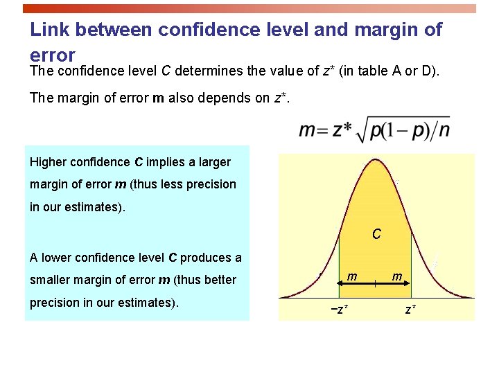
Link between confidence level and margin of error The confidence level C determines the value of z* (in table A or D). The margin of error m also depends on z*. Higher confidence C implies a larger margin of error m (thus less precision in our estimates). C A lower confidence level C produces a smaller margin of error m (thus better precision in our estimates). m −z* m z*

Properties of Confidence Intervals p User chooses the confidence level, C, and hence z* p Margin of error follows from this choice as (z*)(SE of estimator) We want p A high level of confidence p A small margin of error The margin of error is smaller when p z* (and thus the confidence level C) gets smaller p p(1 -p) is smaller p n is larger – this is the usual way to decrease MOE – increase the sample size!

Interpretation of Confidence Intervals p Conditions under which an inference method is valid are never fully met in practice. Exploratory data analysis and judgment should be used when deciding whether or not to use a statistical procedure. p Any individual confidence interval either will or will not contain the true population proportion, p. It is wrong to say that the probability is 95% that the true proportion falls in the confidence interval. p The correct interpretation of a 95% confidence interval is that we are 95% confident that the true proportion falls within the interval. The confidence interval was calculated by a method that gives correct results in ~95% of all possible samples. (See slide #13 above!) In other words, if many such confidence intervals were constructed, ~95% of these intervals would contain the true proportion. HW: Read Introduction to Chapter 6 and Section 6. 1 - 6. 1. 6; do # 6. 3, 6. 5 -6. 9 Previous HW: Read section 5. 5; omit section 5. 6 Do Exercises #5. 85, 5. 87 - 5. 90, 5. 93 -5. 95, 5. 99, 5. 100, 5. 102, 5. 144