6 1 Chapter 6 Probability Distributions The Mc

6 -1 Chapter 6 Probability Distributions © The Mc. Graw-Hill Companies, Inc. , 2000

6 -2 Outline l l 6 -1 Introduction 6 -2 Probability Distributions 6 -3 Mean, Variance, and Expectation 6 -4 The Binomial Distribution © The Mc. Graw-Hill Companies, Inc. , 2000

6 -3 Objectives l l l Construct a probability distribution for a random variable. Find the mean, variance, and expected value for a discrete random variable. Find the exact probability for X successes in n trials of a binomial experiment. © The Mc. Graw-Hill Companies, Inc. , 2000

6 -4 Objectives l Find the mean, variance, and standard deviation for the variable of a binomial distribution. © The Mc. Graw-Hill Companies, Inc. , 2000

6 -2 Probability Distributions 6 -5 l l A variable is defined as a characteristic or attribute that can assume different values. A variable whose values are determined by chance is called a random variable © The Mc. Graw-Hill Companies, Inc. , 2000

6 -2 Probability Distributions 6 -6 l l If a variable can assume only a specific number of values, such as the outcomes for the roll of a die or the outcomes for the toss of a coin, then the variable is called a discrete variable Discrete variables have values that can be counted. © The Mc. Graw-Hill Companies, Inc. , 2000

6 -2 Probability Distributions 6 -7 l l If a variable can assume all values in the interval between two given values then the variable is called a continuous variable. Example - temperature between 680 to 780. Continuous random variables are obtained from data that can be measured rather than counted. © The Mc. Graw-Hill Companies, Inc. , 2000

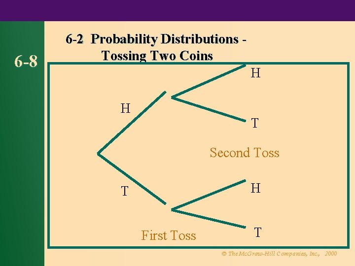
6 -8 6 -2 Probability Distributions Tossing Two Coins H H T Second Toss H T First Toss T © The Mc. Graw-Hill Companies, Inc. , 2000

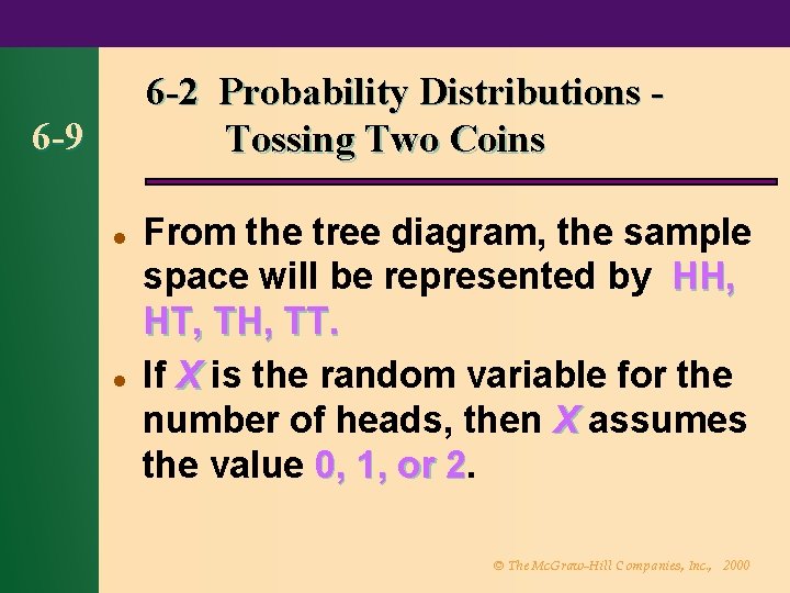
6 -2 Probability Distributions Tossing Two Coins 6 -9 l l From the tree diagram, the sample space will be represented by HH, HT, TH, TT. If X is the random variable for the number of heads, then X assumes the value 0, 1, or 2. 2 © The Mc. Graw-Hill Companies, Inc. , 2000

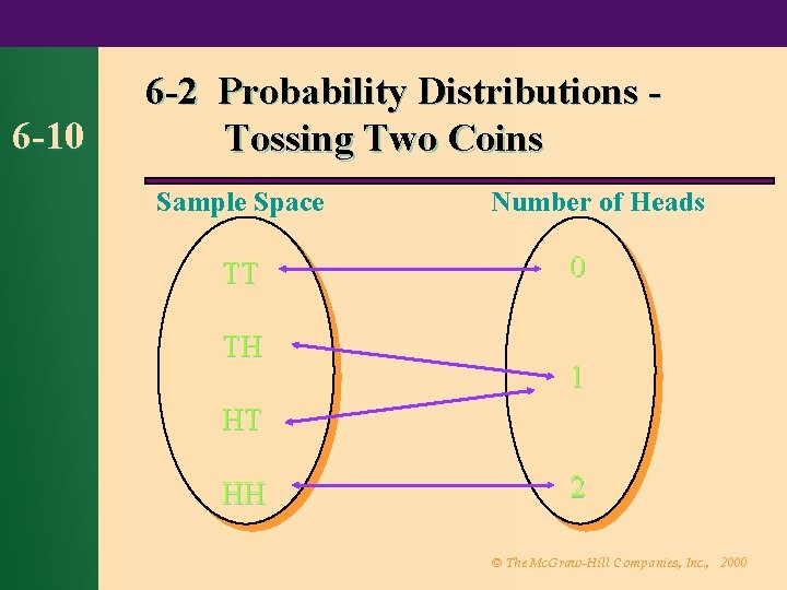
6 -10 6 -2 Probability Distributions Tossing Two Coins Sample Space TT TH Number of Heads 0 1 HT HH 2 © The Mc. Graw-Hill Companies, Inc. , 2000

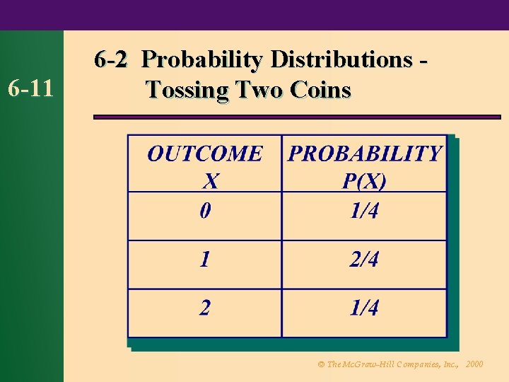
6 -11 6 -2 Probability Distributions Tossing Two Coins © The Mc. Graw-Hill Companies, Inc. , 2000

6 -12 6 -2 Probability Distributions l A probability distribution consists of the values a random variable can assume and the corresponding probabilities of the values. The probabilities are determined theoretically or by observation. © The Mc. Graw-Hill Companies, Inc. , 2000

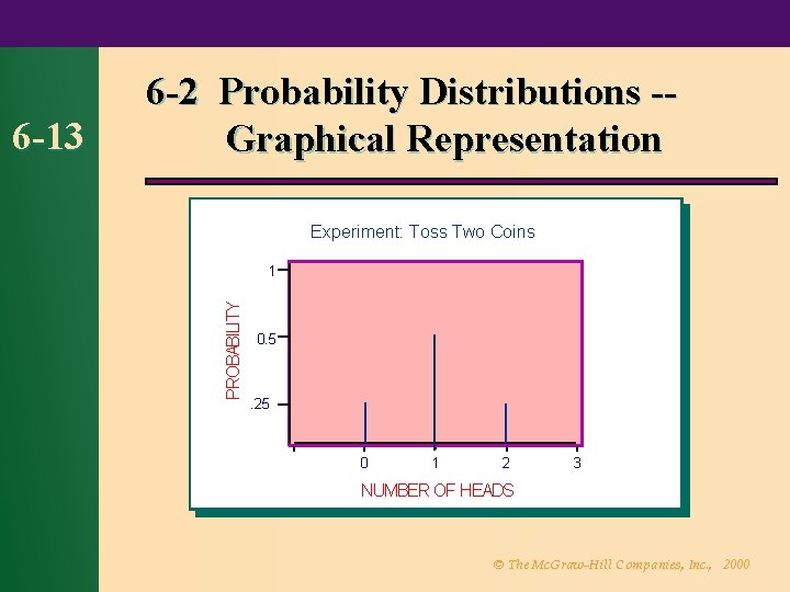
Experiment: Toss Two Coins 1 PROBABILITY 6 -13 6 -2 Probability Distributions -Graphical Representation 0. 5 . 25 0 1 2 3 NUMBER OF HEADS © The Mc. Graw-Hill Companies, Inc. , 2000

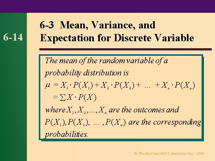
6 -14 6 -3 Mean, Variance, and Expectation for Discrete Variable The mean of the random variable of a probability distribution is = X P( X ) . . . X P( X ) where X , . . . , X are the outcomes and P( X ), . . . , P( X ) are the corresponding probabilities. 1 1 2 2 n n © The Mc. Graw-Hill Companies, Inc. , 2000

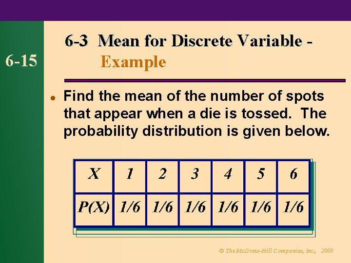
6 -3 Mean for Discrete Variable Example 6 -15 l Find the mean of the number of spots that appear when a die is tossed. The probability distribution is given below. © The Mc. Graw-Hill Companies, Inc. , 2000

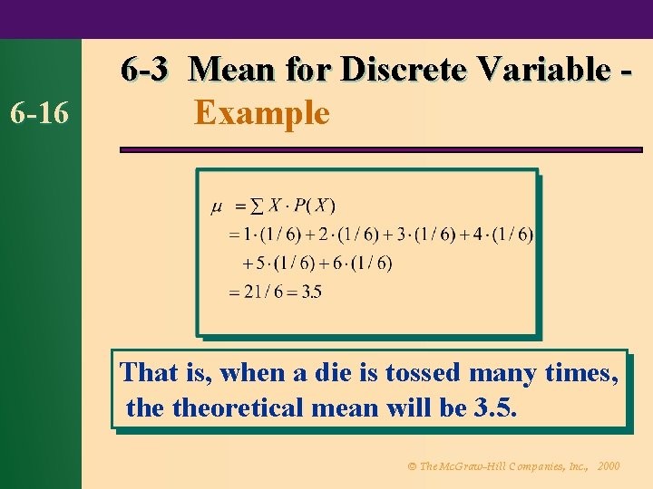
6 -16 6 -3 Mean for Discrete Variable Example That is, when a die is tossed many times, theoretical mean will be 3. 5. © The Mc. Graw-Hill Companies, Inc. , 2000

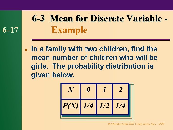
6 -3 Mean for Discrete Variable Example 6 -17 l In a family with two children, find the mean number of children who will be girls. The probability distribution is given below. © The Mc. Graw-Hill Companies, Inc. , 2000

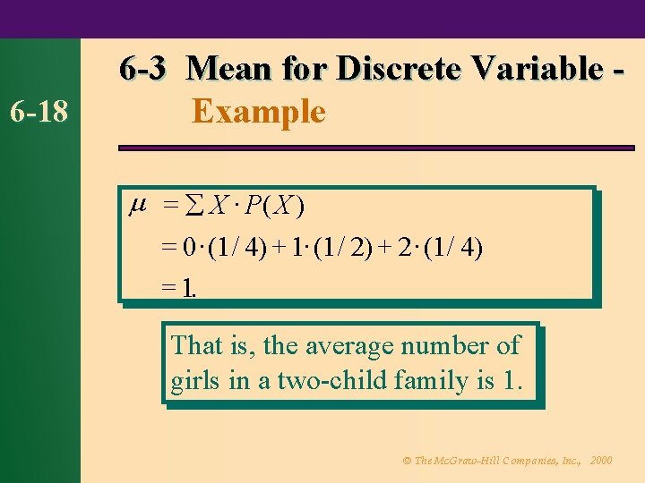
6 -18 6 -3 Mean for Discrete Variable Example X P( X ) 0 (1 / 4) 1 (1 / 2) 2 (1 / 4) = 1. That is, the average number of girls in a two-child family is 1. © The Mc. Graw-Hill Companies, Inc. , 2000

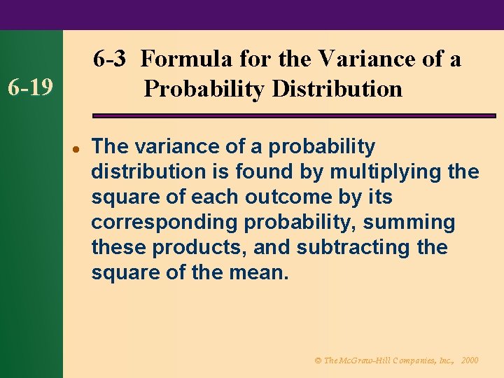
6 -3 Formula for the Variance of a Probability Distribution 6 -19 l The variance of a probability distribution is found by multiplying the square of each outcome by its corresponding probability, summing these products, and subtracting the square of the mean. © The Mc. Graw-Hill Companies, Inc. , 2000

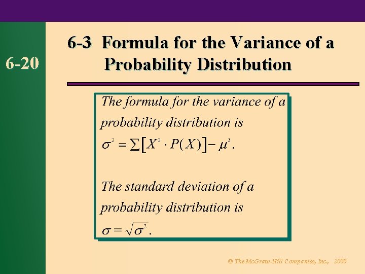
6 -20 6 -3 Formula for the Variance of a Probability Distribution © The Mc. Graw-Hill Companies, Inc. , 2000

6 -3 Variance of a Probability Distribution - Example 6 -21 l The probability that 0, 1, 2, 3, or 4 people will be placed on hold when they call a radio talk show with four phone lines is shown in the distribution below. Find the variance and standard deviation for the data. © The Mc. Graw-Hill Companies, Inc. , 2000

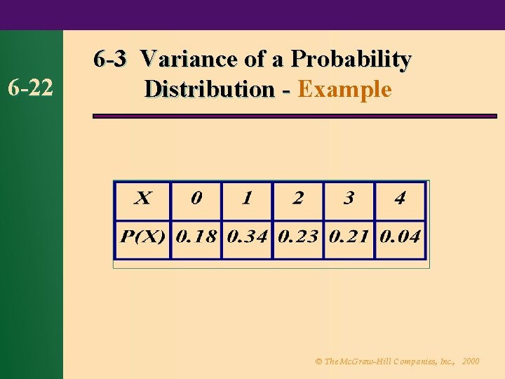
6 -22 6 -3 Variance of a Probability Distribution - Example © The Mc. Graw-Hill Companies, Inc. , 2000

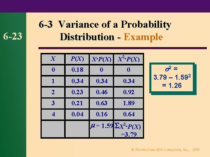
6 -23 6 -3 Variance of a Probability Distribution - Example X P(X) X 2 P(X) X P(X) 0 0. 18 0 0 1 0. 34 2 0. 23 0. 46 0. 92 3 0. 21 0. 63 1. 89 4 0. 04 0. 16 0. 64 2 = 3. 79 – 1. 592 = 1. 26 = 1. 59 X 2 P(X) =3. 79 © The Mc. Graw-Hill Companies, Inc. , 2000

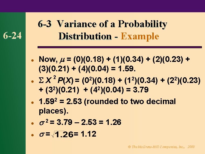
6 -3 Variance of a Probability Distribution - Example 6 -24 l l l Now, = (0)(0. 18) + (1)(0. 34) + (2)(0. 23) + (3)(0. 21) + (4)(0. 04) = 1. 59. X 2 P(X) = (02)(0. 18) + (12)(0. 34) + (22)(0. 23) + (32)(0. 21) + (42)(0. 04) = 3. 79 1. 592 = 2. 53 (rounded to two decimal places). 2 = 3. 79 – 2. 53 = 1. 26 = = 1. 12 © The Mc. Graw-Hill Companies, Inc. , 2000

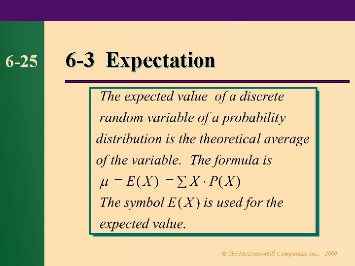
6 -25 6 -3 Expectation © The Mc. Graw-Hill Companies, Inc. , 2000

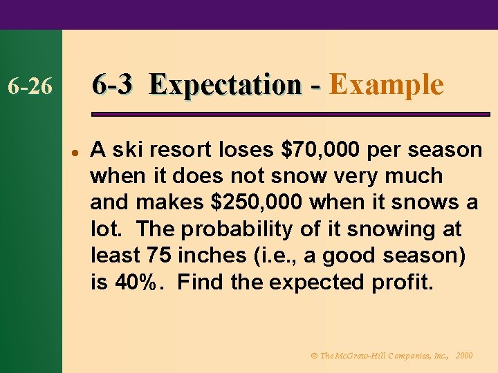
6 -3 Expectation - Example 6 -26 l A ski resort loses $70, 000 per season when it does not snow very much and makes $250, 000 when it snows a lot. The probability of it snowing at least 75 inches (i. e. , a good season) is 40%. Find the expected profit. © The Mc. Graw-Hill Companies, Inc. , 2000

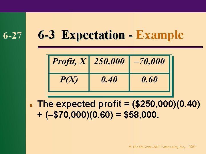
6 -3 Expectation - Example 6 -27 l The expected profit = ($250, 000)(0. 40) + (–$70, 000)(0. 60) = $58, 000. © The Mc. Graw-Hill Companies, Inc. , 2000

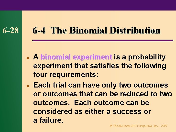
6 -4 The Binomial Distribution 6 -28 l l A binomial experiment is a probability experiment that satisfies the following four requirements: Each trial can have only two outcomes or outcomes that can be reduced to two outcomes. Each outcome can be considered as either a success or a failure. © The Mc. Graw-Hill Companies, Inc. , 2000

6 -4 The Binomial Distribution 6 -29 l l l There must be a fixed number of trials. The outcomes of each trial must be independent of each other. The probability of success must remain the same for each trial. © The Mc. Graw-Hill Companies, Inc. , 2000

6 -4 The Binomial Distribution 6 -30 l The outcomes of a binomial experiment and the corresponding probabilities of these outcomes are called a binomial distribution. © The Mc. Graw-Hill Companies, Inc. , 2000

6 -4 The Binomial Distribution 6 -31 l l l Notation for the Binomial Distribution: P(S) = p, probability of a success P(F) = 1 – p = q, probability of a failure n = number of trials X = number of successes. © The Mc. Graw-Hill Companies, Inc. , 2000

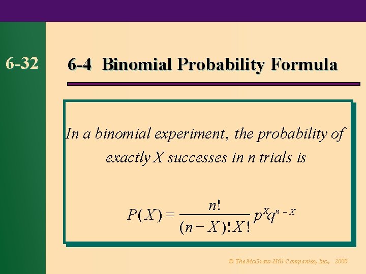
6 -32 6 -4 Binomial Probability Formula In a binomial experiment, the probability of exactly X successes in n trials is n! P( X ) p Xq n X (n X )! X ! © The Mc. Graw-Hill Companies, Inc. , 2000

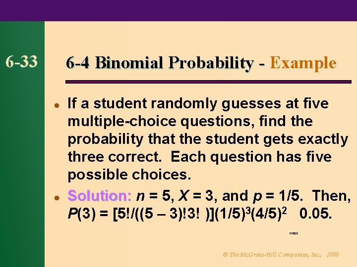
6 -33 6 -4 Binomial Probability - Example l l If a student randomly guesses at five multiple-choice questions, find the probability that the student gets exactly three correct. Each question has five possible choices. Solution: n = 5, X = 3, and p = 1/5. Then, P(3) = [5!/((5 – 3)!3! )](1/5)3(4/5)2 0. 05. © The Mc. Graw-Hill Companies, Inc. , 2000

6 -34 6 -4 Binomial Probability - Example l A survey from Teenage Research Unlimited (Northbrook, Illinois. ) found that 30% of teenage consumers received their spending money from part-time jobs. If five teenagers are selected at random, find the probability that at least three of them will have part -time jobs. © The Mc. Graw-Hill Companies, Inc. , 2000

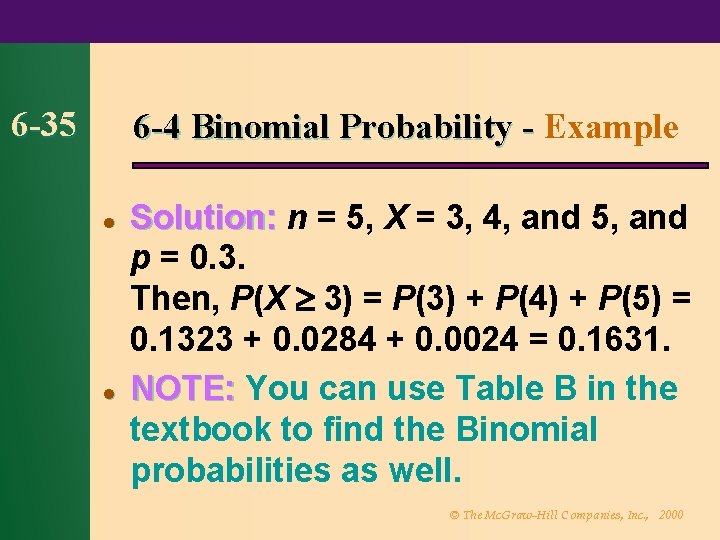
6 -35 6 -4 Binomial Probability - Example l l Solution: n = 5, X = 3, 4, and 5, and p = 0. 3. Then, P(X 3) = P(3) + P(4) + P(5) = 0. 1323 + 0. 0284 + 0. 0024 = 0. 1631. NOTE: You can use Table B in the textbook to find the Binomial probabilities as well. © The Mc. Graw-Hill Companies, Inc. , 2000

6 -36 6 -4 Binomial Probability - Example l A report from the Secretary of Health and Human Services stated that 70% of singlevehicle traffic fatalities that occur on weekend nights involve an intoxicated driver. If a sample of 15 single-vehicle traffic fatalities that occurred on a weekend night is selected, find the probability that exactly 12 involve a driver who is intoxicated. © The Mc. Graw-Hill Companies, Inc. , 2000

6 -37 6 -4 Binomial Probability - Example l Solution: n = 15, X = 12, and p = 0. 7. From Table B, P(X =12) = 0. 170 © The Mc. Graw-Hill Companies, Inc. , 2000

6 -4 Mean, Variance, Standard Deviation for the Binomial Distribution - Example 6 -38 l l l A coin is tossed four times. Find the mean, variance, and standard deviation of the number of heads that will be obtained. Solution: n = 4, p = 1/2, and q = 1/2. = n p = (4)(1/2) = 2. 2 = n p q = (4)(1/2) = 1. = = 1. © The Mc. Graw-Hill Companies, Inc. , 2000