521 Chapter 8 Systems of Linear FirstOrder Differential

521 Chapter 8 Systems of Linear First-Order Differential Equations 註：本章這學期只教不考 另一種解「聯立微分方程式」的方法 (1) Section 4. 9: (2) Chapter 7: (3) Chapter 8: Using matrix operations

522 比較 (1) 這 3 種方法都只適用於 linear & constant coefficients 的情形 註：其實 Laplace transform 可用來解 nonlinear & non-constant coefficient DEs, 但過程頗為複雜 (2) Laplace transform 的方法優於 Section 4 -8 的方法的地方， 在於可以輕易的解決 initial condition 的問題 注意：但是，若 boundary conditions 不是在 t = 0 的地方，用 Laplace transform 需要花一番功夫。

Section 8. 1 Preliminary Theory 524 方法的限制： (a) linear, (b) 1 st order DEs (c) full rank (n 個 dependent variable 需要 n 個式子) 名詞： linear system (pp. 525) homogeneous, nonhomogeneous (pp. 526) solution vector (pp. 526) fundamental set of solutions (pp. 530) general solution (pp. 527) complementary function (pp. 534) particular solution (pp. 534) 本節學習秘訣：和 Section 4 -1 相比較

525 8 -1 -1 表示法和名詞 假設有 n 個 dependent variables x 1(t), x 2(t), ……. , xn(t), n 個只有針對其中一個dependent variable 做微分的 linear DEs : : 稱作 linear system

526 Matrix form of a linear system fn(t) = 0 for all n otherwise solution vector homogeneous linear system nonhomogeneous linear system

527 其中 可改寫成 Example 2 (text page 335) 皆為 的解

528 If x 1(t 0) = r 1, x 2(t 0) = r 2, ………. , xn(t 0) = rn, linear system 可寫成 subject to

8 -1 -2 基本定理 將 Section 4 -1 的幾個定理改成 vector 和 matrix 的型態 [Theorem 8. 1. 1] If the entries of A and F are continuous on a common interval that contains the point t 0, then the initial value problem on the previous page has a unique solution on this interval. (比較 Theorem 4. 1. 1, page 140) 529

[Theorem 8. 1. 2] For the homogeneous linear system (F = 0) if X 1, X 2, …. , Xk are the solution of then is also a solution of [Definition 8. 1. 3 and Theorem 8. 1. 5] If the size of A is n × n and X 1, X 2, …. , Xn are the linearly independent solutions of , then X 1, X 2, …. , Xn are said to be a fundamental set of solutions. Then, the general solution of is c 1, c 2, …. . , cn are arbitrary constants (比較 Theorem 4. 1. 5, page 147) 530

[Theorem 8. 1. 3] Linearly dependent / independent 判斷方式 (課本用 | | 來表示 det) 531

532 Either W(X 1, X 2, …. , Xn) 0 for every t or W(X 1, X 2, …. , Xn) = 0 (比較 Wronskian, page 150) linearly independent

Example 4 (text page 337) determinant 533

[Theorem 8. 1. 6] General solution for nonhomogeneous system subject to 稱作為 complementary function particular solution (比較講義 page 152) 534

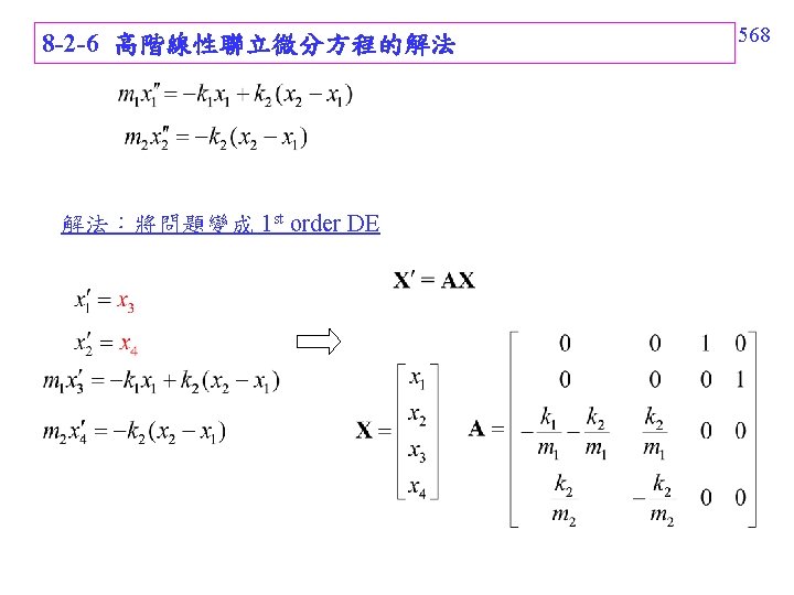
Section 8. 2 Homogeneous Linear Systems 8 -2 -1 本節摘要 (A) 解法的限制： 同講義 page 524 ，但多了二個限制 (d) homogeneous (e) 最好是 constant coefficients 536

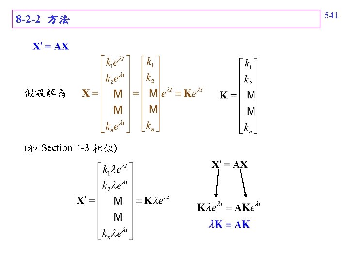
537 (B) 解法 size of A: n × n a = 1, 2, …. , n 假設解為 其中 (constant coefficients) a: A 的 eigenvalue Ka: A 的 eigenvector (AKa = Ka) General solution: 證明見講義 page 541

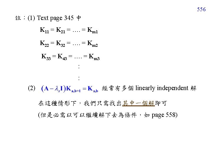
538 (C) 三種情形 Case 1: A has distinct eigenvalues: 解法如前一頁 Case 2: A has repeated eigenvalues 當 a 的 multiplicities 為 m Case 2. 1 可以找到 a 的 m 個 linearly independent eigenvectors 解法同前一頁 Case 2. 2 無法找到 a 的 m 個 linearly independent eigenvectors 若只有 1 個 linearly independent eigenvector，將解表示成 :

539 注意： : Case 2. 3 無法找到 a 的 m 個 linearly independent eigenvectors 有超過 1 個 linearly independent eigenvector 其實，也可以用類似方法求解，但較為複雜

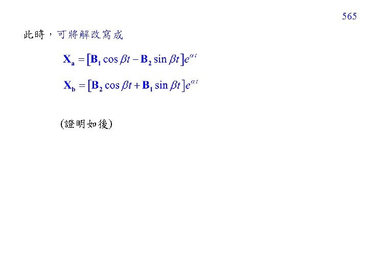
Case 3 若 a = + j 為 A 的eigenvalues, A 為 real matrix b = − j 必為 A 的eigenvalues 若 Ka = B 1 + j. B 2 為 a 所對應的 eigenvector Kb = B 1 − j. B 2 必為 b 所對應的 eigenvector 此時，可將解改寫成 (D) 名詞與其他 multiplicity (page 549) 540

542 的問題變成 (和 linear algebra 當中解 eigenvector, eigenvalue 的問題相同) 是 A 的 eigenvalue K 是 A 的 eigenvector 由 det(A − I) = 0 算出 (稱作 characteristic equation) 當 算出後，K 為使得 成立 的任一個滿足 K 0 的解

543 Example 1 (text page 341) = − 1, 4 (i) When = − 1 k 2 = − k 1 設 k 1 = 1, k 2 = − 1

544 (ii) When = 4 k 2 = 2 k 1/3 設 k 1 = 3, k 2 = 2

545 trajectory y x t (a) Graph of x = e–t + 3 e 4 t Fig. 8. 2. 1 t (b) Graph of y = –e–t + 2 e 4 t

8 -2 -3 Case 1: Distinct Eigenvalues 根據 eigenvalues ，分成 3 cases Case 1: Distinct eigenvalues Case 2: Repeated eigenvalues Case 3: Complex eigenvalues 546

547 Example 2 (text page 343) = − 3, − 4, 5 (distinct)

When = − 3 3 rd row: k 2 = 0 1 st row: −k 1 + k 2 + k 3 = −k 1 + k 3 = 0, k 1 = k 3 When = − 4, = 5 (自己練習解解看) 548

8 -2 -4 Case 2: Repeated Eigenvalues 有時, det(A − I) 會出現 ( − a)m a 被稱作 eigenvalue of multiplicity m (這種情形較複雜，但也是本節的重點) 549

Case 2. 1 當 a 的 multiplicity 為 m (m > 1) 時，有的時候可以將 m 個 linearly independent eigenvectors 全部找出來。 550 此時，solutions 解法和 Case 1 相同 注意： 當 A = AT 時， 若 a 的 multiplicity 為 m ，一定可以找到 a 所對應的 m 個 linearly independent eigenvectors Example 3 (text page 345)

551 (i) 當 = − 1 row operation new 2 nd row = old 2 nd row + 1 st row new 3 rd row = old 3 rd row − 1 st row 3 個 variables, 1 個式子 3− 1=2 2 個 linearly independent solutions

2 個 linearly independent solutions (第一個 solution) 設 k 1 = 0, k 2 = 1 k 3 = 1 (第二個 solution) 設 k 1 = 1, k 2 = 0 k 3 = − 1 Check: 552 的確互為 linearly independent 為 A 在 = − 1 時的 eigenvectors 小技巧： 任意給定其他 n-1 個 unknowns 的值 再將最後一個 unknown 的值算出來 通常可以得到一個新的 independent solution (但是也有的時候得到的解不為 independent, 所以要 check)

553 (ii) 當 = 5 算出來的 eigenvector 為 General solution for Example 3:

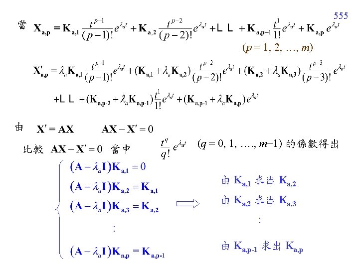
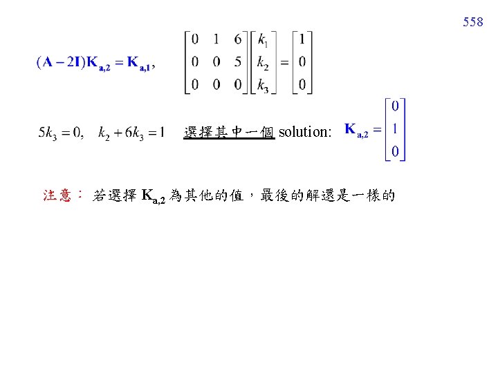
Case 2. 2 當 a 的 multiplicity 為 m (m > 1) 時，有的時候只能找 出 1 個 linearly independent eigenvector Ka, 1。 將 a 所對應的 m 個解表示成 : Ka, 1: 唯一滿足 AKa, 1 = a. Ka, 1 的 eigenvector Ka, q (q 1) 的求法如後頁 554

557 Example 5 (text page 348) eigenvalues: 2, 2, 2 only one independent solution:

559 其中一個 solution: General solution of Example 5

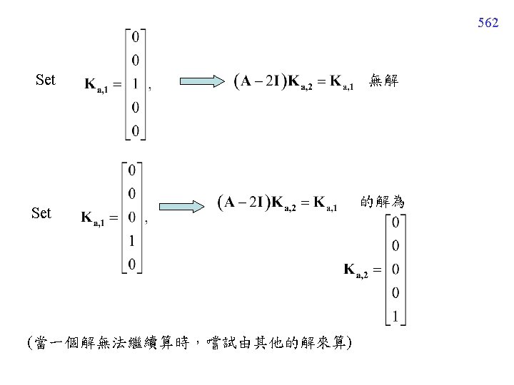
Case 2. 3 當 a 的 multiplicity 為 m (m > 1) 時，有的時候只能找 出 2 ~ m − 1 個 linearly independent eigenvectors 。 例子：Section 8 -2 Exercises 31 and 50 three independent solutions: 560

561 Set k 2 = 1, k 4 = 0 Choose 但 無解

563 General solution for Exercises 31 and 50

8 -2 -5 Case 3: Complex Conjugated Eigenvalues 其實和 Case 1 (distinct eigenvalues) 相同 只是用不同的方式來表示 solutions 當 a = + j 和 b = − j ( , 為 real) 皆為 A 的 eigenvector 且 A 為 real matrix 若 Ka = B 1 + j. B 2 (B 1, B 2 為 real)是 a 所對應的 eigenvector 則 Kb = B 1 − j. B 2 必為是 b 所對應的 eigenvector Proof: 564

566 因此，兩個 linearly independent solutions 可改寫為

Example 6 (text page 351) 已知 = 2 i 為其中一個 eigenvalue，所對應的 eigenvector 為 可以迅速判斷 2 個 independent solutions 為 567

8 -2 -7 Section 8 -2 要注意的地方 (1) 方法適用的情形 (a) linear, (b) 1 st order DEs, (c) full rank (n 個 dependent variable 需要 n 個式子), (d) homogeneous, (e) constant coefficients (2) 複習並熟悉算 eigenvector 的方法 (可以研究快速法) (我們只要得出任何一個 eigenvector 或任何一組 linearly independent eigenvectors 即可，因此可以選擇當中較簡單的 ) (3) Case 2 比較複雜，要多加練習 (4) 注意 page 552 找 independent solution 的小技巧 (5) Case 2. 2 (6)以繼續解下去) 計算前，確定 選擇其中一組解即可 (但是要可 的係數皆為 1 (standard form) 569

570 Section 8. 3 Nonhomogeneous Linear Systems 8. 3. 1 Section 8. 3 摘要 本節討論如何找 的 particular solution (方法 1) undetermined coefficients 猜 particular solutions，類似 Section 4 -4 (方法 2) variation of parameters ，類似 Section 4 -6 (t): fundamental matrix，定義見 page 579

(方法 2) variation of parameters ，with initial conditions 名詞： fundamental matrix (page 579) 571

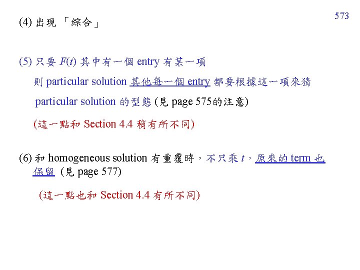
572 8. 3. 2 方法一: Undetermined Coefficients 和 Section 4. 4 的方法相似 根據 F(t) 來「猜」 particular solution 複習講義 page 194 (1) 出現 tn (2) 出現 cos(at) (3) 出現 exp(bt)

574 Example 3 (text page 357) solving the complementary function eigenvalues of A: 2, 4 corresponding eigenvectors for = 2: corresponding eigenvectors for = 4: complementary function

575 解 particular solution 因為 ，所以假設 particular solution 為 注意，每一個 entry 皆有 1, t, e−t From

576

577 補充的範例 (Example 1 in text page 355 的變型) 注意，這一項要保留 設 particular solution 為 乘t

578 choose

8. 3. 3. 1 方法二: Variation of Parameters 先找 complementary function (solution of the associated homogeneous DE) fundamental matrix 579

580 令 由於 每個 column 都是 associated homogeneous DE 的解

581 some constants

Example 4 (text page 359) eigenvalues of A: = − 2, − 5 eigenvectors of A : fundamental matrix 582

583

584 8. 3. 3. 2 和 initial value problems 相結合 在此時，可改寫成定積分的型態 Since thus

8. 3. 4 Section 8. 3 需要注意的地方 (1) 2 × 2 matrix 的 eigenvector 快速算法 (2) 注意 undetermined coefficient 的方法和 Section 4. 4 異同處 (3) Variation of parameters 的部分，關鍵在是否能將公式背起來 (4) 通常 undetermined coefficient 的方法會比較容易解 而 variation of parameters 較複雜，但適用於任何情形 (5) 同樣記得先算 complementary function (homogeneous 部分 的 solution)，再算 particular solution 585

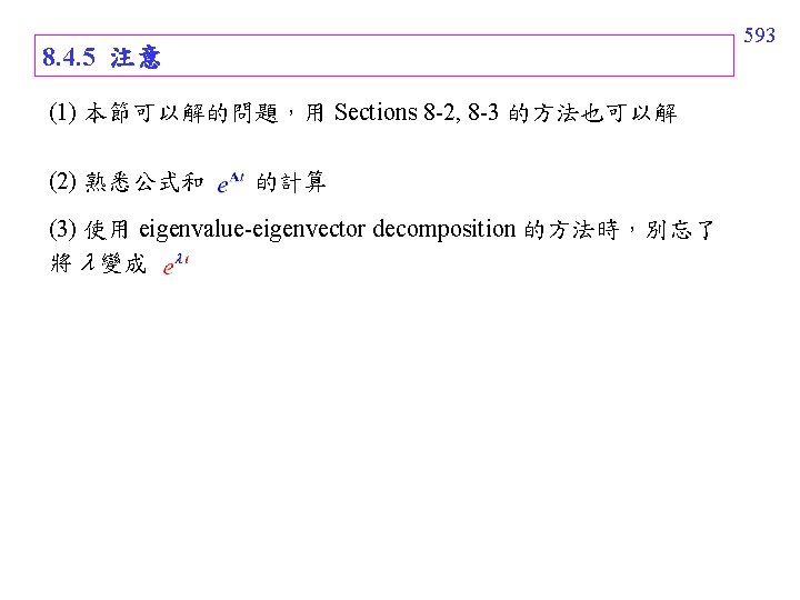
Section 8. 4 Matrix Exponential 8. 4. 1 Section 8. 4 摘要 把 linear system 當成一般 1 st order DE 來解 (比較 Section 2 -3) (1) (2) (3) (With initial condition X(t 0) = X 0) 可以由 Laplace transform (see page 589) 或 eigenvector-eigenvalue decomposition (see page 591) 算出 其中 586

8. 4. 2 For Homogeneous Systems solution: 的定義 h=k− 1 587

8. 4. 3 For Nonhomogeneous Systems solution: 或 比較： with initial conditions 588

8. 4. 4 Computation of 589 一定有這樣的 initial condition 令 X(s) 為 X(t) 的 Laplace transform constant column vector

Example 2 (text page 364) Determine 590

591 殺雞焉用牛刀…… 複習 linear algebra 當中， 的求法 (1) eigenvector-eigenvalue decomposition for A e 1, e 2, e 3, ……, en 皆為 A 的 eigenvectors, 皆為 n × 1 的 column 1, 2, 3 , …. , n 為 e 1, e 2, e 3, ……, en 所對應的eigenvalues

592 例如， Example 1 當中