501 Macroeconomics Chapter 3 Endogenous Growth Prof M

501 Macroeconomics Chapter 3. Endogenous Growth Prof. M. El-Sakka Dept of Economics - Kuwait University

• The models we have seen so far do not provide satisfying answers to our central questions about economic growth. The models’ principal result is a negative one: • - Capital accumulation does not account for a large part of either long-run growth or cross-country income differences. • - The only determinant of income is the “effectiveness of labor” (A), whose exact meaning is not specified and is taken as exogenous. • This chapter focuses on the accumulation of knowledge. • What do we need? • we need to introduce a separate sector of the economy where new ideas are developed.

Framework and Assumptions • We then need to model both how resources are divided between conventional output and new research and development (or R&D) sector, and how inputs into R&D produce new ideas. We make two other major simplifications: • First, both the R&D and goods production functions are assumed to be generalized Cobb–Douglas functions; but the sum of their exponents on the inputs is not necessarily restricted to 1. • Second, the model takes the fraction of output saved and the fractions of the labor force and the capital stock used in the R&D sector as exogenous and constant.

• The model involves four variables: labor (L), capital (K ), technology (A), and output (Y ). • There are two sectors, a goods-producing sector where output is produced an R&D sector where additions to the stock of knowledge are made. Fraction a. L of the labor force is used in the R&D sector and fraction 1−a. L in the goodsproducing sector. Similarly, fraction a. K of the capital stock is used in R&D and the rest in goods production. • Both a. L and a. K are exogenous and constant. • Because the use of an idea or a piece of knowledge in one place does not prevent it from being used elsewhere, both sectors use the full stock of knowledge, A.

• The quantity of output produced at time t is thus • Note that equation (3. 1) implies constant returns to capital and labor: with a given technology, doubling the inputs doubles the amount that can be produced.

• The production of new ideas depends on the quantities of capital and labor engaged in research and on the level of technology. • where B is a shift parameter (determines the position of a function). • Notice that the production function for knowledge is not assumed to have constant returns to scale to capital and labor. Thus it is possible that there are diminishing returns in R&D. At the same time, interactions among researchers, fixed setup costs, and so on may be important enough in R&D that doubling capital and labor more than doubles output. We therefore also allow for the possibility of increasing returns.

• The parameter θ reflects the effect of the existing stock of knowledge on the success of R&D. This effect can operate in either direction. On the one hand, past discoveries may provide ideas and tools that make future discoveries easier. In this case, θ is positive. • On the other hand, the easiest discoveries may be made first. In this case, it is harder to make new discoveries when the stock of knowledge is greater, and so θ is negative. • Because of these conflicting effects, no restriction is placed on θ in (3. 2).

• As in the Solow model, the saving rate is exogenous and constant. In addition, depreciation is set to zero for simplicity. Thus, • Likewise, we continue to treat population growth as exogenous and constant. For simplicity, we do not consider the possibility that it is negative. This implies; • Finally, as in our earlier models, the initial levels of A, K, and L are given and strictly positive. This completes the description of the model.

• Because the model has two state variables whose behavior is endogenous, K and A, it is more complicated to analyze than the Solow model. We therefore begin by considering the model without capital; that is, we set α and β to zero. This case shows most of the model’s central messages. We then turn to the general case.

The Model without Capital • The Dynamics of Knowledge Accumulation • When there is no capital in the model, the production function for output (equation [3. 1]) becomes • Similarly, the production function for new knowledge (equation [3. 2]) is now • Equation (3. 5) implies that output per worker is proportional to A, and thus that the growth rate of output per worker equals the growth rate of A. • We therefore focus on the dynamics of A, which are given by (3. 6). This equation implies that the growth rate of A, denoted g. A, is:

• Taking logs of both sides of (3. 7) and differentiating the two sides with respect to time gives us an expression for the growth rate of g. A: • Multiplying both sides of this expression by g. A(t ) yields • Equation (3. 9) determines the subsequent behavior of g. A.

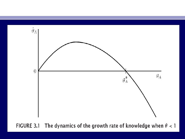
• To describe further how the growth rate of A behaves (and thus to characterize the behavior of output per worker), we must distinguish among the cases θ <1, θ >1, and θ = 1. We discuss each in turn. • • • Case 1: θ < 1 Figure 3. 1 shows the phase diagram for g. A when θ is less than 1. In the diagram and equation (3. 9) for the case of θ < 1, ˙g. A is positive for small positive values of g. A and negative for large values. • We will use g∗A to denote the unique positive value of g. A that implies that ˙g. A is zero.

• From (3. 9), g∗A is defined by: γn + (θ− 1)g∗A = 0. • Solving this for g∗A yields • This analysis implies that regardless of the economy’s initial conditions, g. A converges to g∗A. If the parameter values and the initial values of L and A imply g. A(0) < g∗A, for example, ˙g. A is positive; that is, g. A is rising. It continues to rise until it reaches g∗A.

• Similarly, if g. A(0) > g∗A, then g. A falls until it reaches g∗A. Once g. A reaches g∗A, both A and Y/L grow steadily at rate g∗A. Thus the economy is on a balanced growth path. • The model implies that the long-run growth rate of output per worker, g∗A, is an increasing function of the rate of population growth, n. • Equation (3. 10) also implies that the fraction of the labor force engaged in R&D does not affect long-run growth. This too may seem surprising: since growth is driven by technological progress and technological progress is endogenous, it is natural to expect an increase in the fraction of the economy’s resources devoted to technological progress to increase long-run growth.

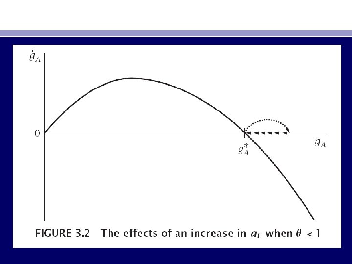
• This change is analyzed in Figure 3. 2. a. L does not enter expression (3. 9) for • ˙g. A: ˙g. A(t) = γng. A(t) + (θ − 1)[˙g. A(t)]2. • Thus the rise in a. L does not affect the curve showing ˙g. A as a function of g. A. But a. L does enter expression (3. 7) for • g. A: g. A(t) = Ba. Lγ L(t)γ A(t )θ− 1. • The increase in a. L therefore causes an immediate increase in g. A but no change in ˙g. A as a function of g. A. This is shown by the dotted arrow in Figure 3. 2.

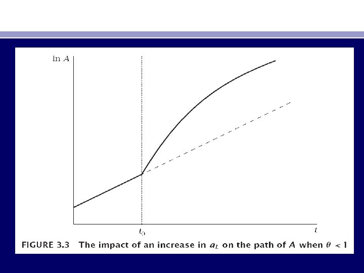
• As the phase diagram shows, the increase in the growth rate of knowledge is not sustained. When g. A is above g∗A, ˙g. A is negative. g. A therefore returns gradually to g∗A and then remains there. Intuitively, the fact that θ is less than 1 means that the contribution of additional knowledge to the production of new knowledge is not strong enough to be self-sustaining. • This analysis implies that, the increase in a. L results in a rise in g. A followed by a gradual return to its initial level. That is, it has a level effect but not a growth effect on the path of A. This information is summarized in Figure 3. 3.

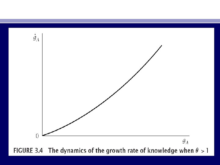
• Case 2: θ > 1 • This corresponds to the case where the production of new knowledge rises more than proportionally with the existing stock. Recall from equation (3. 9) that • ˙g. A = γng. A + (θ − 1)g. A 2. • When θ exceeds 1, this equation implies that ˙g. A is positive for all possible values of g. A. Further, it implies that ˙g. A is increasing in g. A (since g. A must be positive). The phase diagram is shown in Figure 3. 4. • The impact of an increase in the fraction of the labor force engaged in R&D is now dramatic. From Equation (3. 7), an increase in a. L causes an immediate increase in g. A, as before.

` • But ˙g. A is an increasing function of g. A; thus ˙g. A rises as well. And the more rapidly g. A rises, the more rapidly its growth rate rises. Thus the increase in a. L causes the growth rate of A to exceed what it would have been otherwise by an ever-increasing amount.

• Case 3: θ = 1 • When θ is exactly equal to 1, the production of new knowledge is proportional to the stock. In this case, expressions (3. 7) and (3. 9) for g. A and ˙g. A simplify to: • If population growth is positive, g. A is growing over time; in this case the dynamics of the model are similar to those when θ >1. If population growth is zero, on the other hand, g. A is constant regardless of the initial situation.

• The Importance of Population Growth • consider equation (3. 7) for knowledge accumulation: • g. A(t) = Ba. Lγ L(t)γ A(t)θ− 1. 3. 7 • Built into this expression: when there are more people to make discoveries, more discoveries are made. And when more discoveries are made, the stock of knowledge grows faster, and so (all else equal) output person grows faster. In the particular case of θ = 1 and n = 0, this effect operates in a special way: longrun growth is increasing in the level of population. • When θ is greater than 1, the effect is even more powerful, as increases in the level or growth rate of population lead to everrising increases in growth.

• When θ is less than 1, there are decreasing returns to scale to produced factors. In this case, although knowledge may be helpful in generating new knowledge, the generation of new knowledge rises less than proportionally with the existing stock.

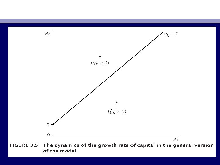
The General Case • The Dynamics of Knowledge and Capital • As mentioned above, when the model includes capital, there are two endogenous state variables, A and K. Paralleling our analysis of the simple model, we focus on the dynamics of the growth rates of A and K. Substituting the production function, (3. 1), into the expression for capital accumulation, (3. 3), yields

• Dividing both sides by K(t) and defining c. K = s (1 − a. K )α(1− a. L)1−α • gives us: • Taking logs of both sides and differentiating with respect to time yields

• g. K is rising if g. A + n − g. K is positive, falling if this expression is negative, and constant if it is zero. • This information is summarized in Figure 3. 5. In (g. A, g. K ) space, the locus of points where g. K is constant has an intercept of n and a slope of 1. Above the locus, g. K is falling; below the locus, it is rising.

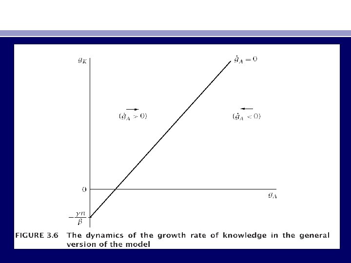
• Similarly, dividing both sides of equation (3. 2), ˙A = B(a. K K)β(a. L L)γAθ, by A yields an expression for the growth rate of A: • where c. A ≡ Ba. K β a. Lγ. Aside from the presence of the Kβ term, this is essentially the same as equation (3. 7) in the simple version of the model. Taking logs and differentiating with respect to time gives

• Thus g. A is rising if βg. K + γ n + (θ− 1)g. A is positive, falling if it is negative, and constant if it is zero. This is shown in Figure 3. 6. The set of points where g. A is constant has an intercept of −γ n/β and a slope of (1− θ)/β. Above this locus, g. A is rising; and below the locus, it is falling.

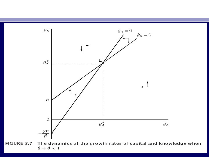
• Case 1: β+θ < 1 • If β + θ is less than 1, (1 − θ)/β is greater than 1. Thus the locus of points where ˙g. A = 0 is steeper than the locus where ˙g. K = 0. This case is shown in Figure 3. 7. The initial values of g. A and g. K are determined by the parameters of the model and by the initial values of A, K, and L. Their dynamics are then as shown in the figure. • Figure 3. 7 shows that regardless of where g. A and g. K begin, they converge to Point E in the diagram. Both ˙g. A and ˙g. K are zero at this point. Thus the values of g. A and g. K at Point E, which we denote g∗A and g∗K , must satisfy

The Nature of Knowledge and the Determinants of the Allocation of Resources to R&D • So far we have simply described the “A” variable produced by R&D as knowledge. But knowledge comes in many forms. • Many of these different types of knowledge play important roles in economic growth. Imagine, for example, that 100 years ago there had been a halt to basic scientific progress, or to the invention of applied technologies. it seems likely that all of them would have led to substantial reductions in growth. • There is no reason to expect the determinants of the accumulation of these different types of knowledge to be the same. There is thus no reason to expect a unified theory of the growth of knowledge. Rather, we should expect to find various factors underlying the accumulation of knowledge.

The Nature of Knowledge and the Determinants of the Allocation of Resources to R&D • At the same time, all types of knowledge share one essential feature: they are nonrival. That is, the use of an item of knowledge in one application makes its use by someone else no more difficult. • Conventional private economic goods, in contrast, are rival: the use of, say, an item of clothing by one individual precludes its simultaneous use by someone else. • In the case of knowledge, excludability depends both on the nature of the knowledge itself and on economic institutions governing property rights. Patent laws, for example, give inventors rights over the use of their designs and discoveries. Under a different set of laws, inventors’ ability to prevent the use of their discoveries by others might be smaller.

The Nature of Knowledge and the Determinants of the Allocation of Resources to R&D • In some cases, excludability is more dependent on the nature of the knowledge and less dependent on the legal system. The recipe for Coca-Cola is sufficiently complex that it can be kept secret without copyright or patent protection. • The degree of excludability is likely to have a strong influence on how the development and allocation of knowledge depart from perfect competition. If a type of knowledge is entirely nonexcludable, there can be no private gain in its development. • When knowledge is excludable, the producers of new knowledge can license the right to use the knowledge at positive prices, and hence hope to earn positive returns on their R&D efforts. •

The Nature of Knowledge and the Determinants of the Allocation of Resources to R&D • The major forces governing the allocation of resources to the development of knowledge are four forces: 1. support for basic scientific research, 2. private incentives for R&D and innovation, 3. alternative opportunities for talented individuals, and 4. learningby-doing. • • 1. Support for Basic Scientific Research Basic scientific knowledge are available relatively freely; this research is not motivated by the desire to earn private returns in the market. The economics of this type of knowledge are relatively straightforward. Since it is useful in production and is given away at zero cost, it has a positive externality. Thus its production should be subsidized.

The Nature of Knowledge and the Determinants of the Allocation of Resources to R&D • 2. Private Incentives for R&D and Innovation • Many innovations receive little or no external support and are motivated almost entirely by the desire for private gain. • As described above, for R&D to result from economic incentives, the knowledge that is created must be at least somewhat excludable. Thus the developer of a new idea has some degree of market power. • Typically, the developer is modeled as having exclusive control over the use of the idea and as licensing its use to the producers of final goods.

The Nature of Knowledge and the Determinants of the Allocation of Resources to R&D • There are in fact three distinct externalities from R&D: the consumer-surplus effect, the business-stealing effect, and the R&D effect. – The consumer-surplus effect is that the individuals or firms licensing ideas from innovators obtain some surplus, since innovators cannot engage in perfect price discrimination. Thus this is a positive externality from R&D. – The business-stealing effect is that the introduction of a superior technology typically makes existing technologies less attractive, and therefore harms the owners of those technologies. This externality is negative.

The Nature of Knowledge and the Determinants of the Allocation of Resources to R&D – The R&D effect is that innovators are generally assumed not to control the use of their knowledge in the production of additional knowledge. Innovators are assumed to earn returns on the use of their knowledge in goods production (equation [3. 1]) but not in knowledge production (equation [3. 2]). Thus the development of new knowledge has a positive externality on others engaged in R&D. • The net effect of these three externalities is ambiguous. It is generally believed, however, that the normal situation is for the overall externality from R&D to be positive. In this case the equilibrium level of R&D is inefficiently low, and R&D subsidies can increase welfare.

The Nature of Knowledge and the Determinants of the Allocation of Resources to R&D • 3. Alternative Opportunities for Talented Individuals • Major innovations and advances in knowledge are often the result of the work of extremely talented individuals. Such individuals typically have choices other than just pursuing innovations and producing goods. • Hence economic incentives and social forces influencing the activities of highly talented individuals may be important to the accumulation of knowledge. • three factors that influence talented individuals’ decisions whether to pursue activities. • 1. the size of the relevant market: the larger is the market from which a talented individual can reap returns, the greater are the incentives to enter a given activity.

The Nature of Knowledge and the Determinants of the Allocation of Resources to R&D • 2. the degree of diminishing returns. • 3. the ability to keep the returns from one’s activities

• 4. Learning-by-Doing • All inputs are now engaged in goods production; thus the production function becomes • The simplest case of learning-by-doing is when learning occurs as a side effect of the production of new capital, the stock of knowledge is a function of the stock of capital. Thus there is only one state variable. • To analyze this economy, begin by substituting (3. 23) into (3. 22). This yields:

• Remember before that the key determinant of the economy’s dynamics is how θ compares with 1, equivalent is how φ compares with 1. • If φ is less than 1, the long-run growth rate of the economy is a function of n. • If φ is greater than 1, there is explosive growth. • if φ equals 1, there is explosive growth if n is positive and steady growth if n equals 0.

• Empirical Application: Time-Series Tests of Endogenous Growth Models • Jones (1995 b) raises a critical issue about these models: Does growth in fact vary with the factors identified by the models in the way the models predict? • Jones considers two approaches to testing the predictions of fully endogenous growth models about changes in growth. • The first starts with the observation that the models predict that changes in the models’ parameters permanently affect growth. • For example, in the model of Section 3. 3 with β + θ =1 and n = 0, changes in s, a. L, and a. K change the economy’s long run growth rate.

• He therefore asks whether the actual growth rate of income person is stationary or non-stationary and considers several tests of stationarity versus non-stationarity. • A simple one is to regress the growth rate of income person, on a constant and a trend, and then test the null hypothesis that b = 0.

• A second test is an augmented Dickey-Fuller test. Consider a regression of the form • If growth has some normal level that it reverts to when it is pushed away, ρ is negative. If it does not, ρ is 0. • Jones examines data on U. S. income person over the period 1880– 1987. His statistical results seem to provide powerful evidence that growth is stationary. • The augmented Dickey-Fuller test overwhelmingly rejects the null hypothesis that ρ = 0, thus appearing to indicate stationarity. •

• The Magnitudes and Correlates of Changes in Long-Run Growth • Jones’s second approach is to examine the relationships between the determinants of growth identified by endogenous growth models and actual growth rates. • He begins by considering learning-by-doing models with φ = 1. Recall that model yields a relationship of the form • This implies that the growth rate of income person is

• where gx denotes the growth rate of x. g. K is given by • where s is the fraction of output that is invested and δ is the depreciation rate. • Jones observes that Y/K, δ, and g. L all both appear to be fairly steady, while investment rates have been trending up. Thus the model predicts an upward trend in growth. • Jones reports that in most major industrialized countries, Y/K is about 0. 4 and the ratio of investment to GDP has been rising by about 1% per decade.

• Empirical Application: Population Growth and Technological Change since 1 Million B. C. • Kremer (1993), argues that endogenous growth provide insights into the dynamics of population, technology, and income over the broad sweep of human history. • Kremer begins his analysis by noting that essentially all models of the endogenous growth of knowledge predict that technological progress is an increasing function of population size. • He then argues that over almost all of human history, technological progress has led mainly to increases in population rather than increases in output person.

• A Simple Model • Kremer’s formal model is a straightforward. First, output depends on technology, labor, and land: • where T denotes the fixed stock of land. • Second, additions to knowledge are proportional to population, and also depend on the stock of knowledge:

• And third, population adjusts so that output person equals the subsistence level, denoted y: • Aside from this Malthusian assumption about the determination of population, γ = 1. • We solve the model in two steps. The first is to find the size of the population that can be supported on the fixed stock of land at a given time. Substituting expression (3. 57) for output into the Malthusian population condition, (3. 59), yields

• Solving this condition for L(t ) gives us • This equation states that the population that can be supported is decreasing in the subsistence level of output, increasing in technology, and proportional to the amount of land. • The second step is to find the dynamics of technology and population. Since both y and T are constant, (3. 61) implies that the growth rate of L is (1 − α)/α times the growth rate of A:

• Thus in this case, (3. 62) implies that the growth rate of population is proportional to the level of population. • Thus population growth is increasing in the size of the population unless α is large or θ is much less than 1 (or a combination of the two). Intuitively, Kremer’s model implies increasing growth even with diminishing returns to knowledge in the production of new knowledge (that is, even with θ <1) • because labor is now a produced factor: improvements in technology lead to higher population, which in turn leads to further improvements in technology.

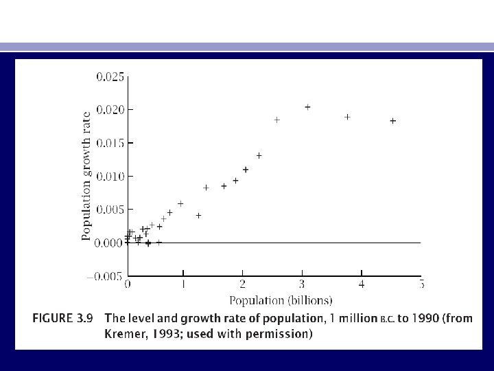
• Kremer tests the model’s predictions using population estimates extending back to 1 million B. C. that have been constructed by archaeologists and anthropologists. • • Figure 3. 9 shows the resulting scatter plot of population growth against population. Each observation shows the level of population at the beginning of some period and the average annual growth rate of population over that period. • • The figure shows a strongly positive, and approximately linear, relationship between population growth and the level of population. A regression of growth on a constant and population (in billions) yields

• A regression of growth on a constant and population (in billions) yields • where n is population growth and L is population, and where the numbers in parentheses are standard errors. • Thus there is an overwhelmingly statistically significant association between the level of population and its growth rate.

• Population Growth versus Growth in Income per Person over the Very Long Run • As described above, over nearly all of history technological progress has led almost entirely to higher population rather than to higher average income. • But this has not been true over the past few centuries: the enormous technological progress of the modern era has led not only to vast population growth, but also to vast increases in average income.

• Income and population growth rise very slowly, but almost all of technological progress is reflected in higher population rather than higher average income. • But when population becomes large enough that technological progress is relatively rapid, this no longer occurs; instead, a large fraction of the effect of technological progress falls on average income rather than on population. • A further extension of the demographic assumptions leads to additional implications. The evidence suggests that preferences are such that once average income is sufficiently high, population growth is decreasing in income. the model predicts that population growth peaks at some point and then declines.

• Models of Knowledge Accumulation and the Central Questions of Growth Theory • Our analysis of economic growth is motivated by two issues: the growth over time in standards of living, and their disparities across different parts of the world. • What the models of R&D and knowledge accumulation have to say about these issues?

• Explaining cross-country income differences on the basis of differences in knowledge accumulation faces a fundamental problem, however: the nonrivalry of knowledge. • Thus there is no inherent reason that producers in poor countries cannot use the same knowledge as producers in rich countries. If the relevant knowledge is publicly available, poor countries can become rich by having their workers or managers read the appropriate literature. • And if the relevant knowledge is proprietary knowledge produced by private R&D, poor countries can become rich by instituting a credible program for respecting foreign firms’ property rights.

• With such a program, the firms in developed countries with proprietary knowledge would open factories in poor countries, hire their inexpensive labor, and produce output using the proprietary technology. The result would be that the marginal product of labor in poor countries, and hence wages, would rapidly rise to the level of developed countries. • There are numerous examples of poor regions or countries, ranging from European colonies over the past few centuries to many countries today, where foreign investors can establish plants and use their know-how with a high degree of confidence that the political environment will be relatively stable, their plants will not be nationalized, and their profits will not be taxed at exorbitant rates. Yet we do not see incomes in those areas jumping to the levels of industrialized

• One might object to this argument on the grounds that in practice the flow of knowledge is not instantaneous. In fact, however, this does not resolve the difficulties with attributing cross-country income differences to differences in knowledge. • If economies but do not all have access to the same technology, the lags in the diffusion of knowledge from rich to poor countries that are needed to account for observed differences in incomes are extremely long—on the order of a century or more. • It is hard to believe that the reason that some countries are so poor is that they do not have access to the improvements in technology that have occurred over the past century.

• One may also object on the grounds that the difficulty countries face is not lack of access to advanced technology, but lack of ability to use the technology. • But this objection implies that the main source of differences in standards of living is not different levels of knowledge or technology, but differences in whatever factors allow richer countries to take better advantage of technology. Understanding differences in incomes therefore requires understanding the reasons for the differences in these factors.