5 Sediment transport models JSSBIO 1 Huttula Lecture

5. Sediment transport models JSSBIO 1 Huttula Lecture Set 4 1

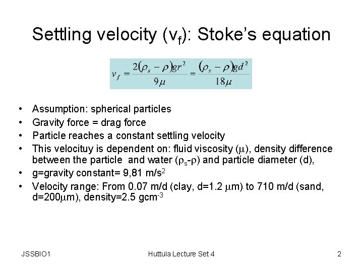
Settling velocity (vf): Stoke’s equation • • Assumption: spherical particles Gravity force = drag force Particle reaches a constant settling velocity This velocituy is dependent on: fluid viscosity ( ), density difference between the particle and water ( s- ) and particle diameter (d), • g=gravity constant= 9, 81 m/s 2 • Velocity range: From 0. 07 m/d (clay, d=1. 2 m) to 710 m/d (sand, d=200 m), density=2. 5 gcm-3 JSSBIO 1 Huttula Lecture Set 4 2

Settling speed in nature • Particles are seldom spherical: clay particles are like plates • Aggregation of particles happens due to the electromagnetic forces cohesive soils (clays, mud…) • Organic compounds like humic substances have a very fragile structure changes even in water column • velocity from Stoke’s equation has to be corrected with empirical relations • Baba& Komar, 1981: vreal=0. 761 vf • In sediment transport models vf is calculated using the median particle size from a surface sediment sample JSSBIO 1 Huttula Lecture Set 4 3

Erosion or resuspension from bottom • • • Acting forces on a particle laying on the bottom 1. difference between gravity on buoyancy 2. drag force by the current 3. lifting force due to the pressure differences as caused by water flowing between particles 4. electromagnetic forces causing aggregation Term 1. density difference and particle (diameter)3 Terms 2 and 3. shear force caused by current and particle (diameter)2 Shields’s empirical curve for erosion in design of structures A simplified erosion curve by Hjulström (erosion vs. current velocity) In models we use most often the critical shear concept JSSBIO 1 Huttula Lecture Set 4 4

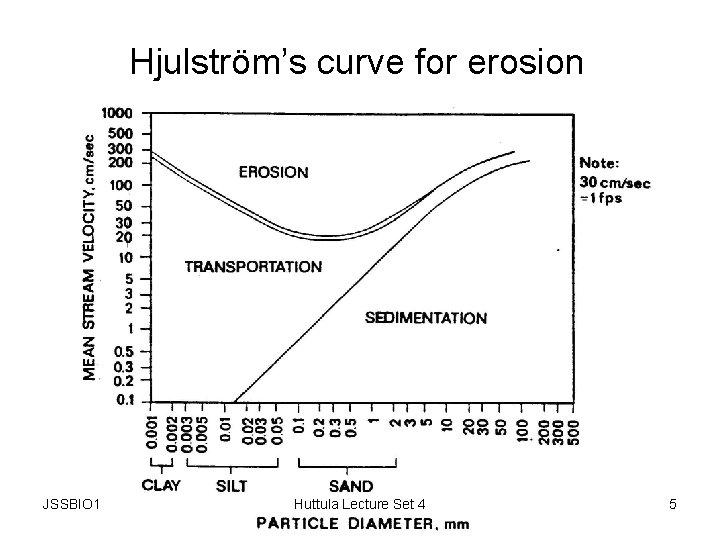
Hjulström’s curve for erosion JSSBIO 1 Huttula Lecture Set 4 5

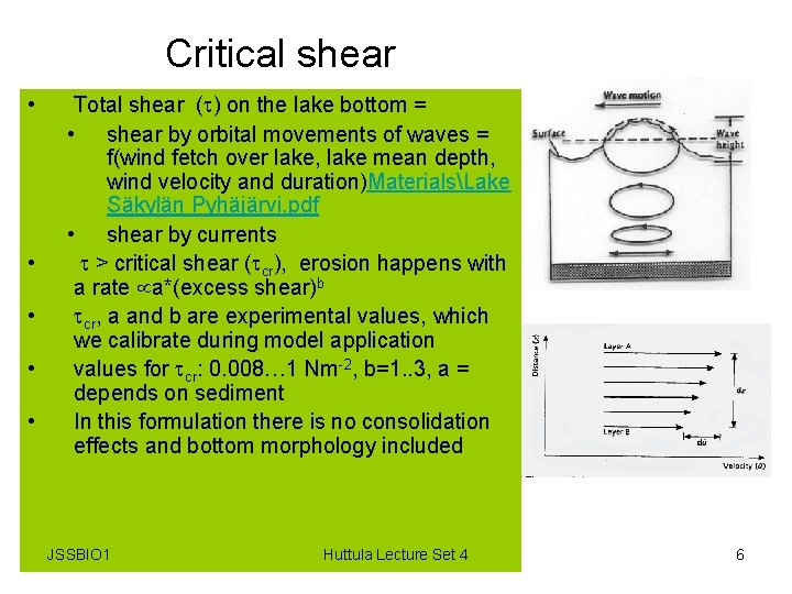
Critical shear • • • Total shear ( ) on the lake bottom = • shear by orbital movements of waves = f(wind fetch over lake, lake mean depth, wind velocity and duration)MaterialsLake Säkylän Pyhäjärvi. pdf • shear by currents > critical shear ( cr), erosion happens with a rate a*(excess shear)b cr, a and b are experimental values, which we calibrate during model application values for cr: 0. 008… 1 Nm-2, b=1. . 3, a = depends on sediment In this formulation there is no consolidation effects and bottom morphology included JSSBIO 1 Huttula Lecture Set 4 6

Calculation of sediment transport • Simple screening tools: http: //el. erdc. usace. army. mil/dots/doer/tools. html • Using numerical flow models for predicting the horizontal current field • Suspended solids concentration is calculated with concentration equation • Following terms in concentration equation: – – – JSSBIO 1 advection with settling speed in vertical dimension turbulence mass flow from tributaries and to out flowing river settling and deposition to bottom erosion or resuspension from bottom Huttula Lecture Set 4 7

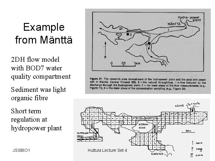
Example from Mänttä 2 DH flow model with BOD 7 water quality compartment Sediment was light organic fibre Short term regulation at hydropower plant JSSBIO 1 Huttula Lecture Set 4 8

Example from Karhijärvi • Three different models were tested 2 DH, 2 DV and 3 D model • Models were tested in an runoff case in Oct 1992, when heavy rains caused erosion from watershed and a heavy suspended solids load to lake • Data: winds on the lake, water current observations, turbidity observations • 3 D model gave best results JSSBIO 1 Huttula Lecture Set 4 9

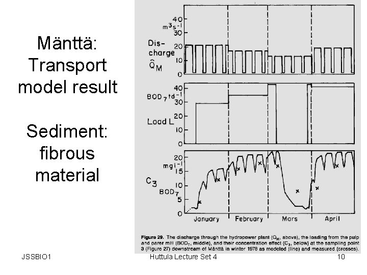
Mänttä: Transport model result Sediment: fibrous material JSSBIO 1 Huttula Lecture Set 4 10

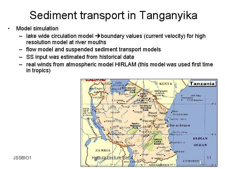
Sediment transport in Tanganyika • Model simulation – lake wide circulation model boundary values (current velocity) for high resolution model at river mouths – flow model and suspended sediment transport models – SS input was estimated from historical data – real winds from atmospheric model HIRLAM (this model was used first time in tropics) JSSBIO 1 Huttula Lecture Set 4 11

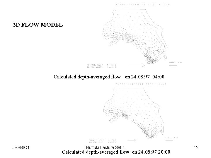
3 D FLOW MODEL Calculated depth-averaged flow on 24. 08. 97 04: 00. JSSBIO 1 Huttula Lecture Set 4 Calculated depth-averaged flow on 24. 08. 97 20: 00 12

3 D SEDIMENT TRANSPORT MODEL (A), 12: 00 24. 08. 97 (B) 0: 00 28. 08. 97 (C) after 22, 82 and 166 hours after the simulation start respectively. JSSBIO 1 Huttula Lecture Set 4 13

6. Water quality models JSSBIO 1 Huttula Lecture Set 4 14

JSSBIO 1 Huttula Lecture Set 4 15

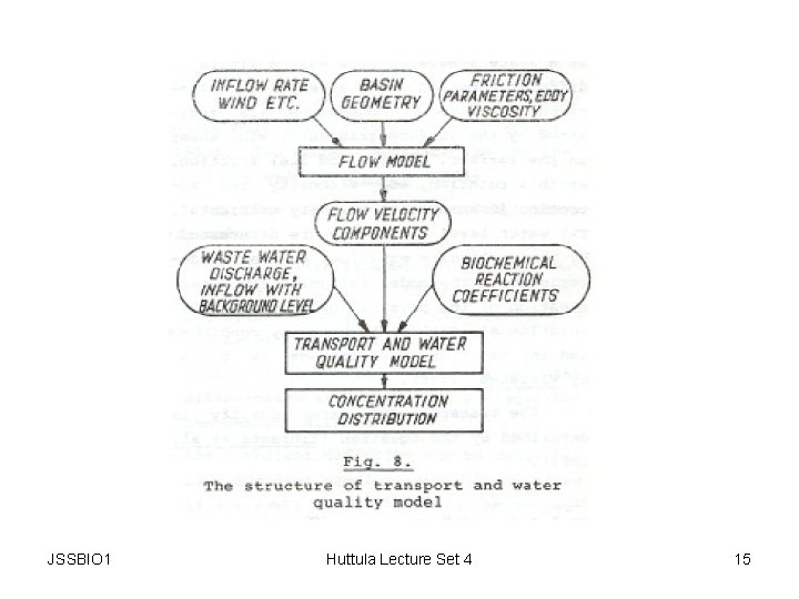
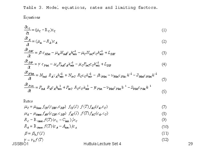
Concentration equation where, – c = concentration, q. L= amount of loading release , n= length measure against release, u, v, w = x-, y- ja z- advective velocities in x-, y- ja zdirections, Dx, Dy, Dz = dispersion coefficients, R(T, c) = biogeochemical changes in concentration JSSBIO 1 Huttula Lecture Set 4 16

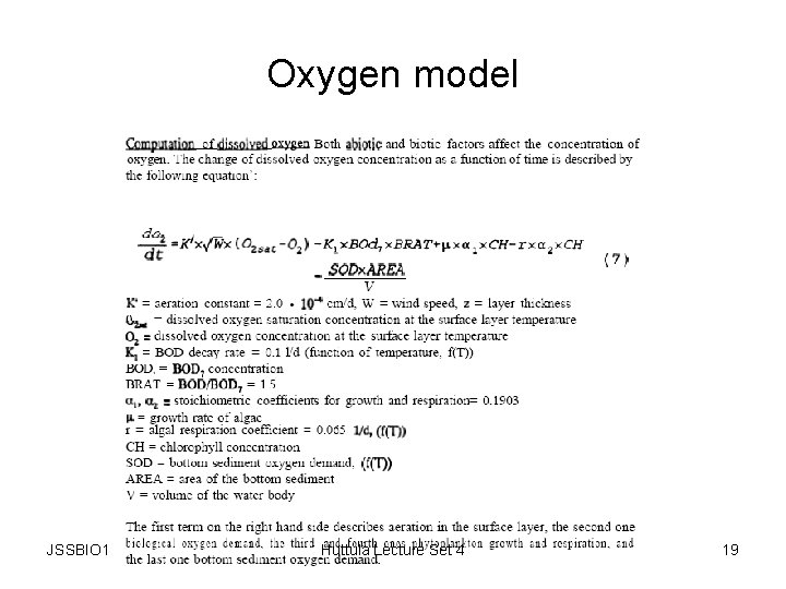
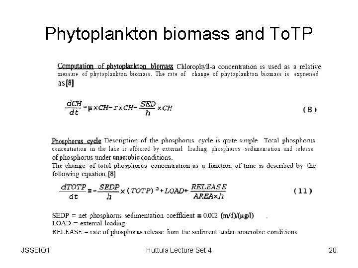
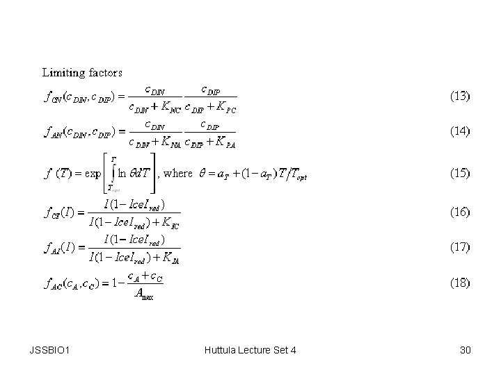
Application of WQ-models • We include : – Advection – Dispersion – Settling on the bottom • Bio- chemical processes – Decomposition, respiration, aeration, anaerobic release of P from the bottom – Select the most important variables concerning the problem – Oxygen, nutrients (like P, N), chlorophyll-a and some conservative substance (like Na) – Limiting factors (light, nutrients, …) must be included. Check! – Temperature corrections must be included. Check! JSSBIO 1 Huttula Lecture Set 4 17

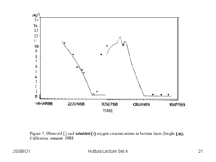
Lake Lappajärvi WQ-model • PROBE temperature model – MaterialsEffects of Climate Change. . pdf • PROBE-WQ model – MaterialsLappajarvi_WQ. pdf JSSBIO 1 Huttula Lecture Set 4 18

Oxygen model JSSBIO 1 Huttula Lecture Set 4 19

Phytoplankton biomass and To. TP JSSBIO 1 Huttula Lecture Set 4 20

JSSBIO 1 Huttula Lecture Set 4 21

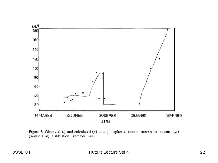
JSSBIO 1 Huttula Lecture Set 4 22

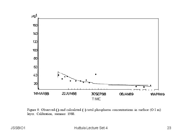
JSSBIO 1 Huttula Lecture Set 4 23

JSSBIO 1 Huttula Lecture Set 4 24

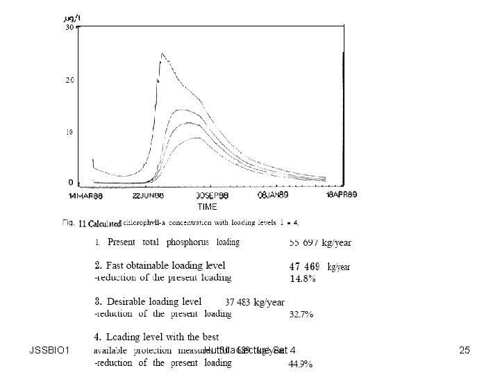
JSSBIO 1 Huttula Lecture Set 4 25

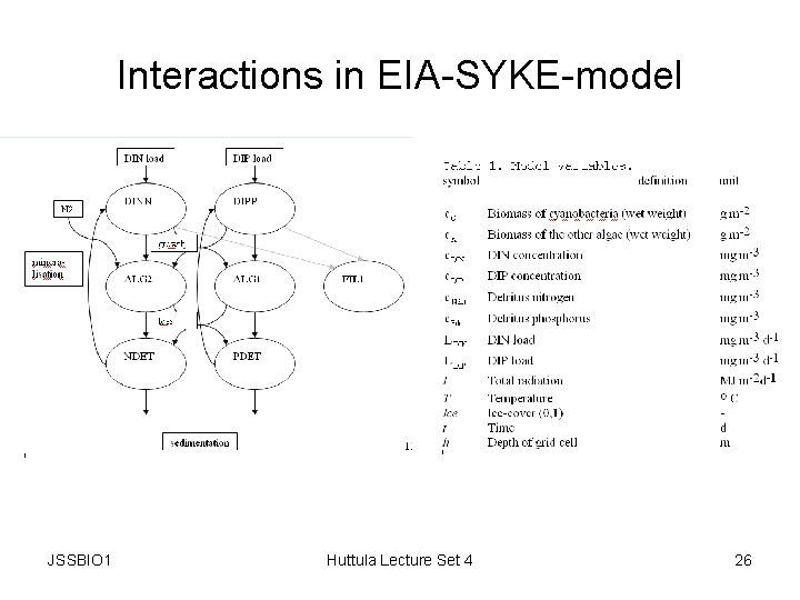
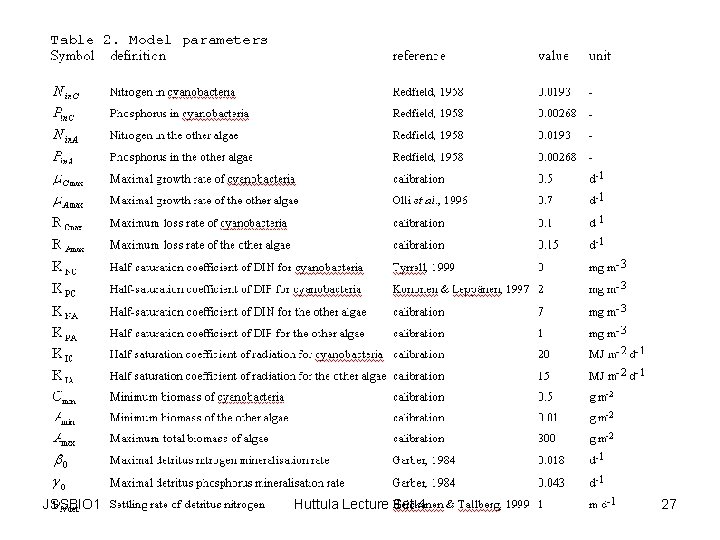
Interactions in EIA-SYKE-model JSSBIO 1 Huttula Lecture Set 4 26

JSSBIO 1 Huttula Lecture Set 4 27

JSSBIO 1 Huttula Lecture Set 4 28

JSSBIO 1 Huttula Lecture Set 4 29

JSSBIO 1 Huttula Lecture Set 4 30

Other WQ-model applications • Several case studies MaterialsFlow_and_WQ_Models_Sarkkula. pdf • Lake Pyhäselkä – MaterialsPyhaselka. pdf • What happened to WQ after real reduction of loads? – MaterialsIAWQ 99. pdf JSSBIO 1 Huttula Lecture Set 4 31

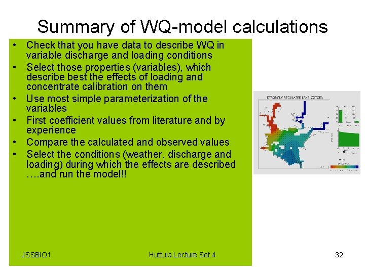
Summary of WQ-model calculations • Check that you have data to describe WQ in variable discharge and loading conditions • Select those properties (variables), which describe best the effects of loading and concentrate calibration on them • Use most simple parameterization of the variables • First coefficient values from literature and by experience • Compare the calculated and observed values • Select the conditions (weather, discharge and loading) during which the effects are described …. and run the model!! JSSBIO 1 Huttula Lecture Set 4 32