5 Introduction to estimation A B C D

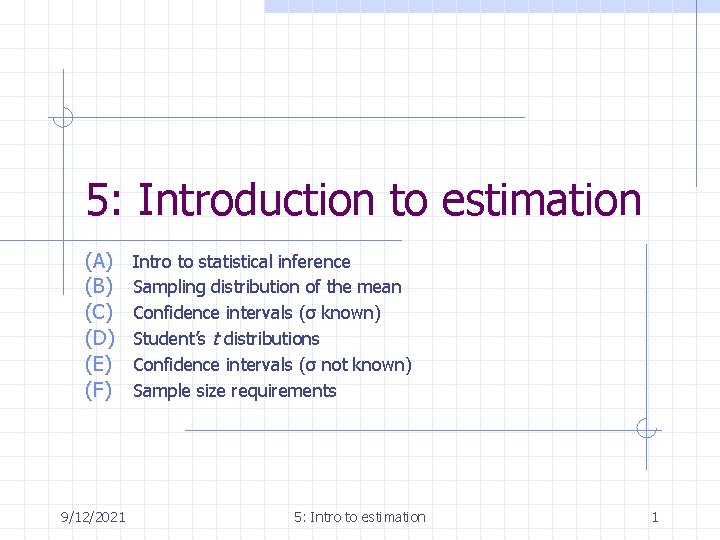
5: Introduction to estimation (A) (B) (C) (D) (E) (F) 9/12/2021 Intro to statistical inference Sampling distribution of the mean Confidence intervals (σ known) Student’s t distributions Confidence intervals (σ not known) Sample size requirements 5: Intro to estimation 1

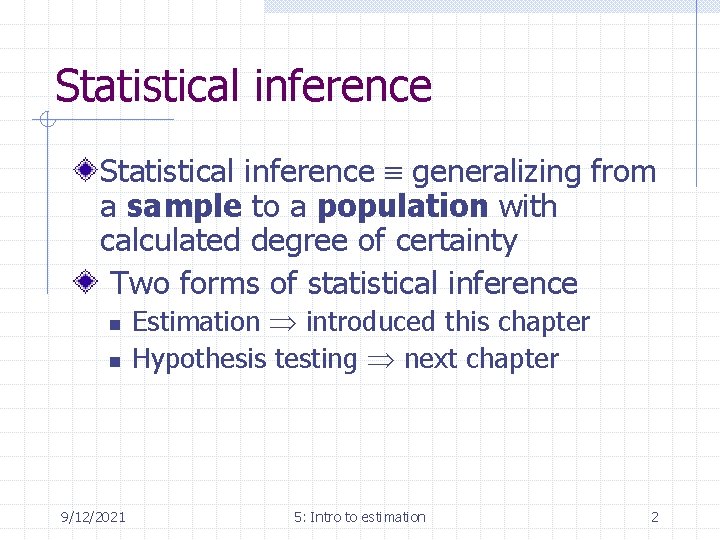
Statistical inference generalizing from a sample to a population with calculated degree of certainty Two forms of statistical inference n n 9/12/2021 Estimation introduced this chapter Hypothesis testing next chapter 5: Intro to estimation 2

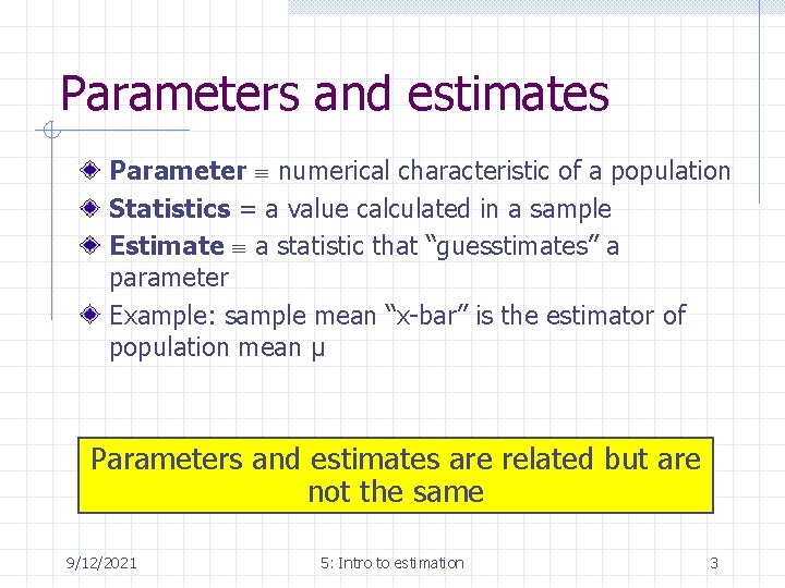
Parameters and estimates Parameter numerical characteristic of a population Statistics = a value calculated in a sample Estimate a statistic that “guesstimates” a parameter Example: sample mean “x-bar” is the estimator of population mean µ Parameters and estimates are related but are not the same 9/12/2021 5: Intro to estimation 3

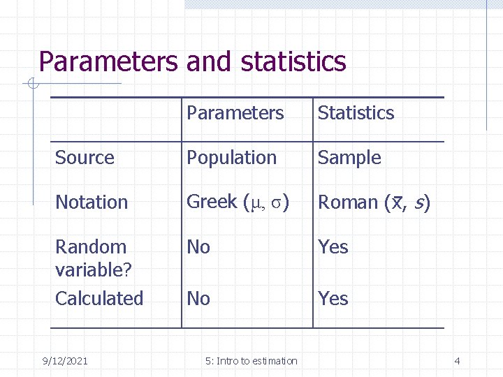
Parameters and statistics Parameters Statistics Source Population Sample Notation Greek (μ, σ) Roman (x, s) Random variable? Calculated No Yes 9/12/2021 5: Intro to estimation 4

Sampling distribution of the mean x-bar takes on different values with repeated (different) samples µ remain constant Even though x-bar is variable, it’s “behavior” is predictable The behavior of x-bar is predicted by its sampling distribution, the Sampling Distribution of the Mean (SDM) 9/12/2021 5: Intro to estimation 5

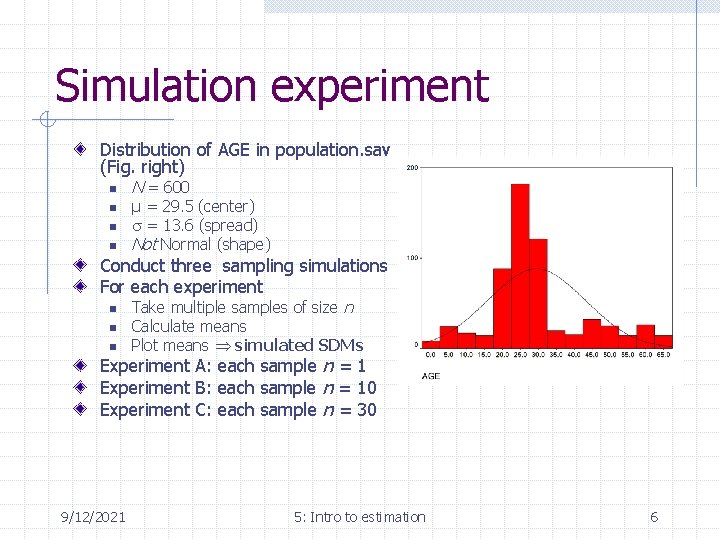
Simulation experiment Distribution of AGE in population. sav (Fig. right) n n N = 600 µ = 29. 5 (center) s = 13. 6 (spread) Not Normal (shape) Conduct three sampling simulations For each experiment n n n Take multiple samples of size n Calculate means Plot means simulated SDMs Experiment A: each sample n = 1 Experiment B: each sample n = 10 Experiment C: each sample n = 30 9/12/2021 5: Intro to estimation 6

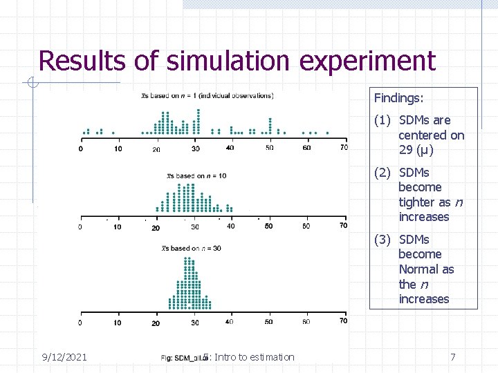
Results of simulation experiment Findings: (1) SDMs are centered on 29 (µ) (2) SDMs become tighter as n increases (3) SDMs become Normal as the n increases 9/12/2021 5: Intro to estimation 7

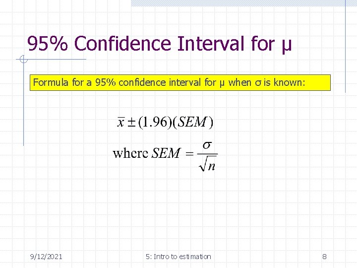
95% Confidence Interval for µ Formula for a 95% confidence interval for μ when σ is known: 9/12/2021 5: Intro to estimation 8

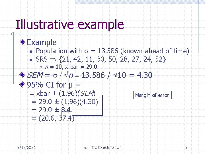
Illustrative example Example n n Population with σ = 13. 586 (known ahead of time) SRS {21, 42, 11, 30, 50, 28, 27, 24, 52} w n = 10, x-bar = 29. 0 SEM = s / n = 13. 586 / 10 = 4. 30 95% CI for µ = = xbar ± (1. 96)(SEM) = 29. 0 ± (1. 96)(4. 30) = 29. 0 ± 8. 4 = (20. 6, 37. 4) 9/12/2021 5: Intro to estimation Margin of error 9

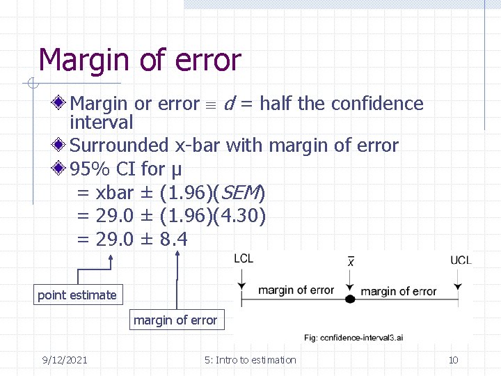
Margin of error Margin or error d = half the confidence interval Surrounded x-bar with margin of error 95% CI for µ = xbar ± (1. 96)(SEM) = 29. 0 ± (1. 96)(4. 30) = 29. 0 ± 8. 4 point estimate margin of error 9/12/2021 5: Intro to estimation 10

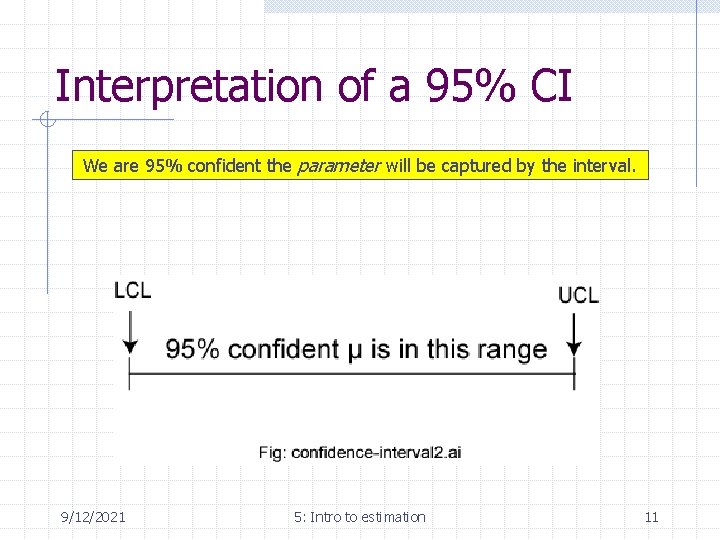
Interpretation of a 95% CI We are 95% confident the parameter will be captured by the interval. 9/12/2021 5: Intro to estimation 11

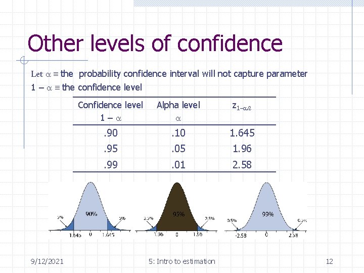
Other levels of confidence Let a the probability confidence interval will not capture parameter 1 – a the confidence level 9/12/2021 Confidence level 1–a Alpha level a z 1–a/2 . 90 . 10 1. 645 . 95 . 05 1. 96 . 99 . 01 2. 58 5: Intro to estimation 12

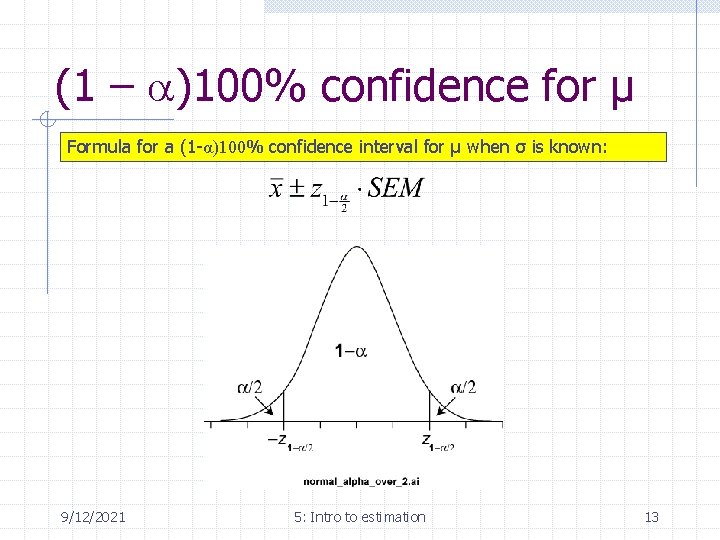
(1 – a)100% confidence for μ Formula for a (1 -α)100% confidence interval for μ when σ is known: 9/12/2021 5: Intro to estimation 13

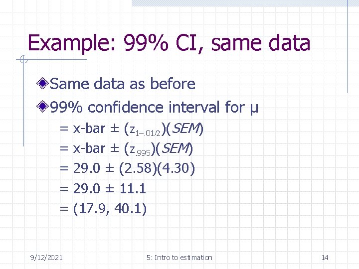
Example: 99% CI, same data Same data as before 99% confidence interval for µ = = = 9/12/2021 x-bar ± (z 1–. 01/2)(SEM) x-bar ± (z. 995)(SEM) 29. 0 ± (2. 58)(4. 30) 29. 0 ± 11. 1 (17. 9, 40. 1) 5: Intro to estimation 14

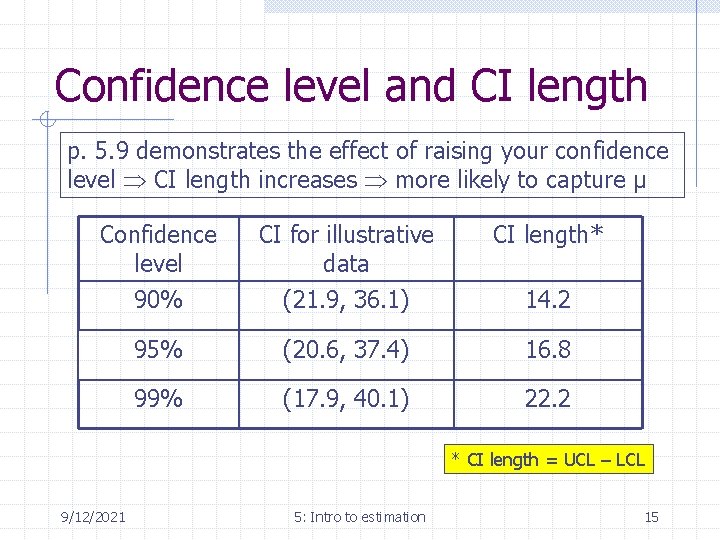
Confidence level and CI length p. 5. 9 demonstrates the effect of raising your confidence level CI length increases more likely to capture µ Confidence level CI for illustrative data CI length* 90% (21. 9, 36. 1) 14. 2 95% (20. 6, 37. 4) 16. 8 99% (17. 9, 40. 1) 22. 2 * CI length = UCL – LCL 9/12/2021 5: Intro to estimation 15

Beware Prior CI formula applies only to n n n SRS Normal SDMs σ known ahead of time It does not account for: n n 9/12/2021 GIGO Poor quality samples (e. g. , due to nonresponse) 5: Intro to estimation 16

When σ is Not Known In practice we rarely know σ Instead, we calculate s and use this as an estimate of σ This adds another element of uncertainty to the inference A modification of z procedures called Student’s t distribution is needed to account for this additional uncertainty 9/12/2021 5: Intro to estimation 17

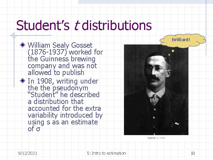
Student’s t distributions William Sealy Gosset (1876 -1937) worked for the Guinness brewing company and was not allowed to publish In 1908, writing under the pseudonym “Student” he described a distribution that accounted for the extra variability introduced by using s as an estimate of σ 9/12/2021 5: Intro to estimation Brilliant! 18

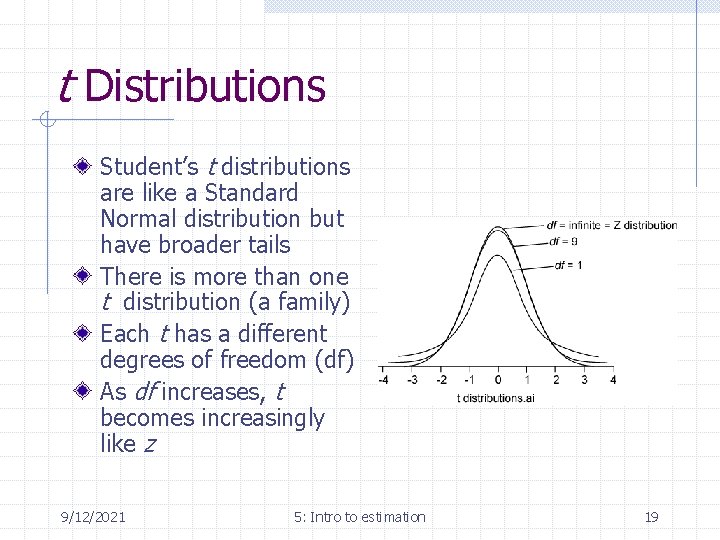
t Distributions Student’s t distributions are like a Standard Normal distribution but have broader tails There is more than one t distribution (a family) Each t has a different degrees of freedom (df) As df increases, t becomes increasingly like z 9/12/2021 5: Intro to estimation 19

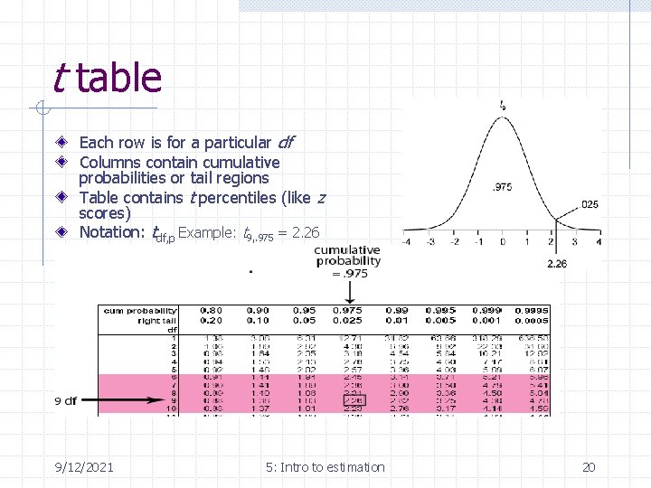
t table Each row is for a particular df Columns contain cumulative probabilities or tail regions Table contains t percentiles (like z scores) Notation: tdf, p Example: t 9, . 975 = 2. 26 9/12/2021 5: Intro to estimation 20

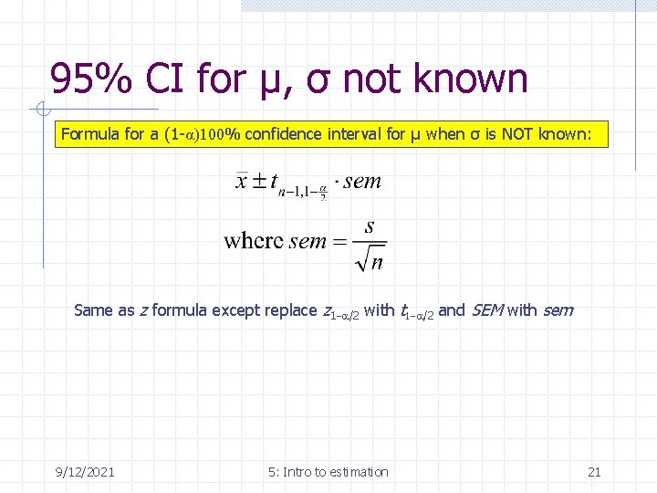
95% CI for µ, σ not known Formula for a (1 -α)100% confidence interval for μ when σ is NOT known: Same as z formula except replace z 1 -a/2 with t 1 -a/2 and SEM with sem 9/12/2021 5: Intro to estimation 21

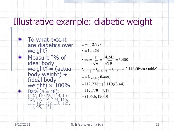
Illustrative example: diabetic weight To what extent are diabetics over weight? Measure “% of ideal body weight” = (actual body weight) ÷ (ideal body weight) × 100% Data (n = 18): {107, 119, 99, 114, 120, 104, 88, 114, 124, 116, 101, 121, 152, 100, 125, 114, 95, 117} 9/12/2021 5: Intro to estimation 22

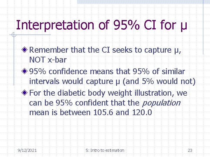
Interpretation of 95% CI for µ Remember that the CI seeks to capture µ, NOT x-bar 95% confidence means that 95% of similar intervals would capture µ (and 5% would not) For the diabetic body weight illustration, we can be 95% confident that the population mean is between 105. 6 and 120. 0 9/12/2021 5: Intro to estimation 23

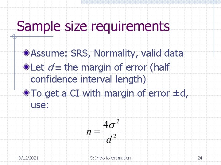
Sample size requirements Assume: SRS, Normality, valid data Let d the margin of error (half confidence interval length) To get a CI with margin of error ±d, use: 9/12/2021 5: Intro to estimation 24

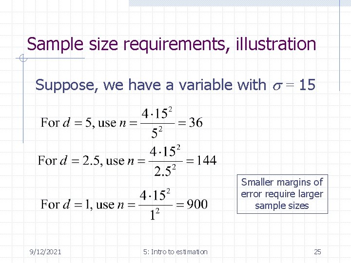
Sample size requirements, illustration Suppose, we have a variable with s = 15 Smaller margins of error require larger sample sizes 9/12/2021 5: Intro to estimation 25

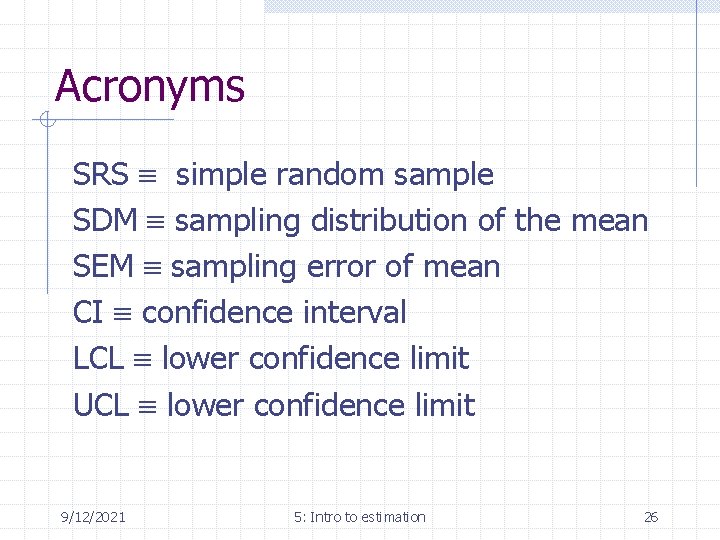
Acronyms SRS simple random sample SDM sampling distribution of the mean SEM sampling error of mean CI confidence interval LCL lower confidence limit UCL lower confidence limit 9/12/2021 5: Intro to estimation 26