5 FEKS 05 TREES Unit4 FREE ELECTIVE Data

![procedure heapsort (T[1. . n]) { T is an array to be sorted } procedure heapsort (T[1. . n]) { T is an array to be sorted }](https://slidetodoc.com/presentation_image_h2/847c1e775db22c5a09cc9ca80daa7644/image-24.jpg)
![Page# 165 procedure shift-down (T[1. . n], i) { This procedure shifts node i Page# 165 procedure shift-down (T[1. . n], i) { This procedure shifts node i](https://slidetodoc.com/presentation_image_h2/847c1e775db22c5a09cc9ca80daa7644/image-25.jpg)
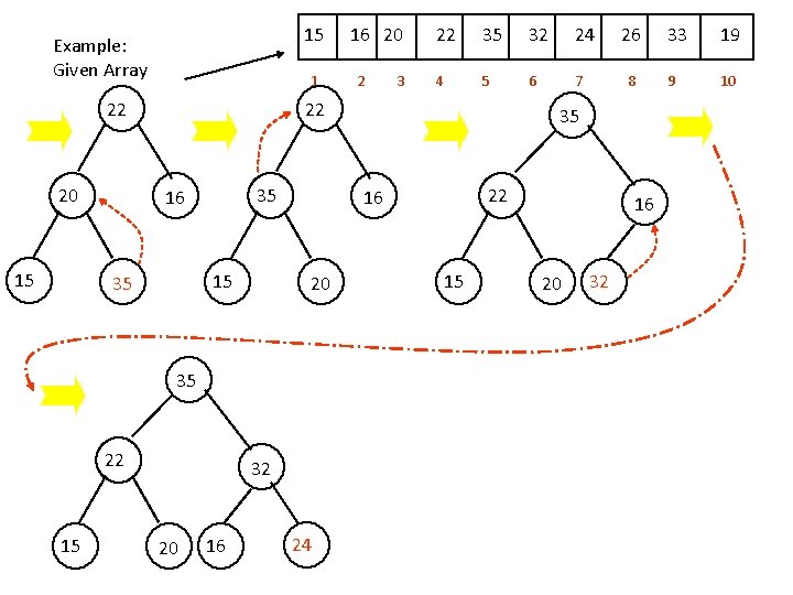
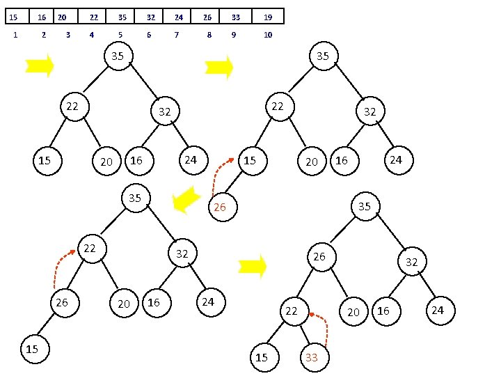
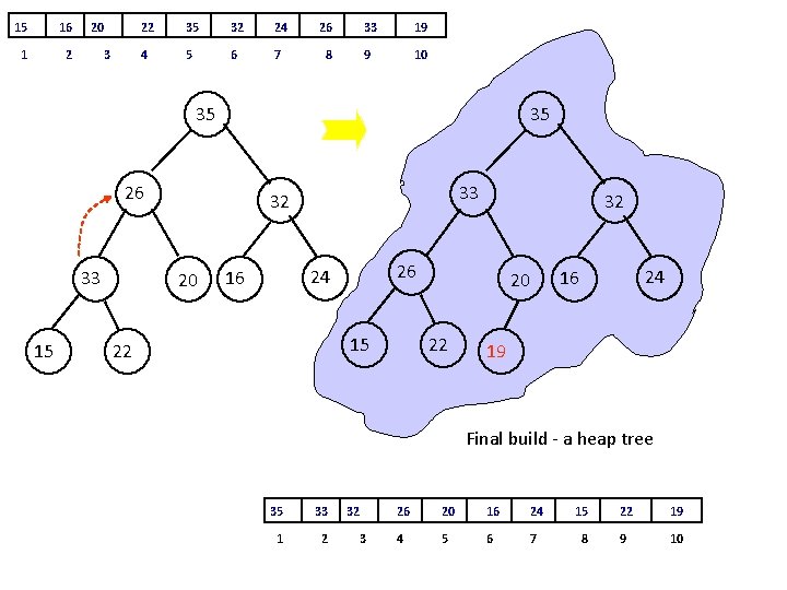
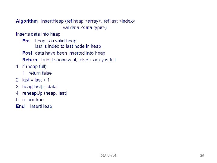
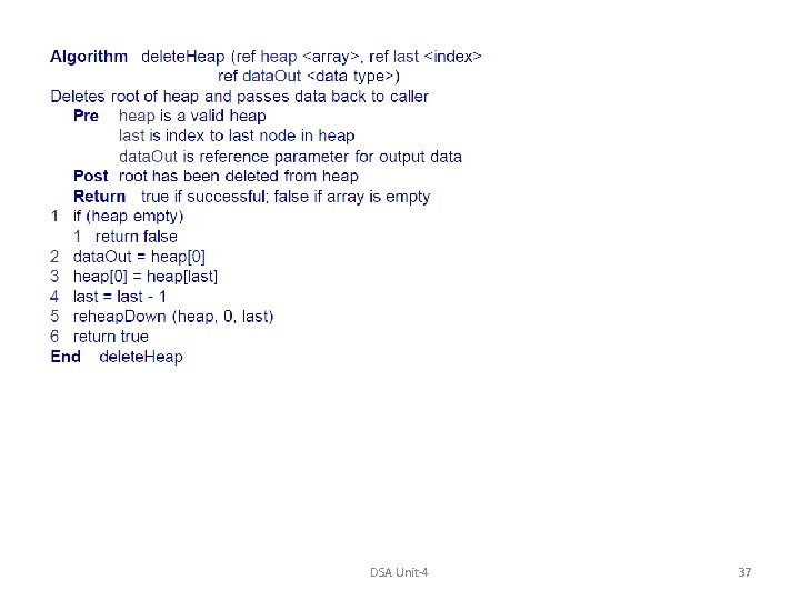
![procedure heapsort (T[1. . n]) { T is an array to be sorted } procedure heapsort (T[1. . n]) { T is an array to be sorted }](https://slidetodoc.com/presentation_image_h2/847c1e775db22c5a09cc9ca80daa7644/image-38.jpg)
![procedure heapsort (T[1. . n]) { T is an array to be sorted } procedure heapsort (T[1. . n]) { T is an array to be sorted }](https://slidetodoc.com/presentation_image_h2/847c1e775db22c5a09cc9ca80daa7644/image-39.jpg)
- Slides: 47

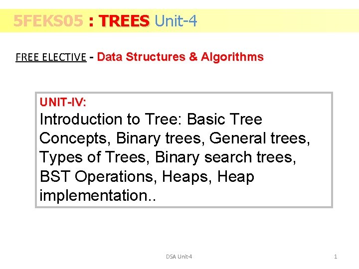
5 FEKS 05 : TREES Unit-4 FREE ELECTIVE - Data Structures & Algorithms UNIT-IV: Introduction to Tree: Basic Tree Concepts, Binary trees, General trees, Types of Trees, Binary search trees, BST Operations, Heap implementation. . DSA Unit-4 1

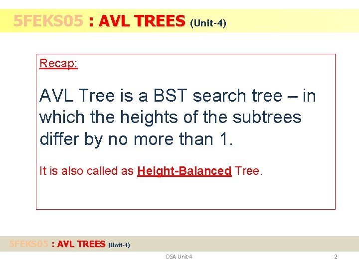
5 FEKS 05 : AVL TREES (Unit-4) Recap: AVL Tree is a BST search tree – in which the heights of the subtrees differ by no more than 1. It is also called as Height-Balanced Tree. 5 FEKS 05 : AVL TREES (Unit-4) DSA Unit-4 2

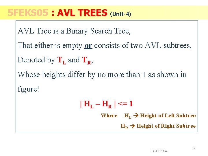
5 FEKS 05 : AVL TREES (Unit-4) AVL Tree is a Binary Search Tree, That either is empty or consists of two AVL subtrees, Denoted by TL and TR, Whose heights differ by no more than 1 as shown in figure! | HL – HR | <= 1 Where HL Height of Left Subtree HR Height of Right Subtree DSA Unit-4 3

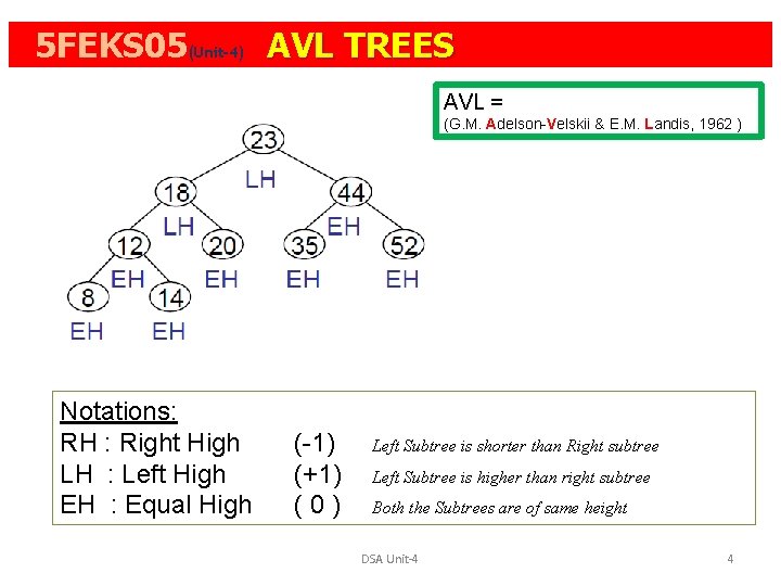
5 FEKS 05(Unit-4): AVL TREES AVL = (G. M. Adelson-Velskii & E. M. Landis, 1962 ) Notations: RH : Right High LH : Left High EH : Equal High (-1) (+1) (0) Left Subtree is shorter than Right subtree Left Subtree is higher than right subtree Both the Subtrees are of same height DSA Unit-4 4

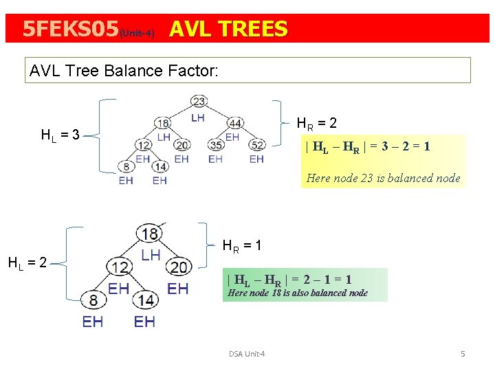
5 FEKS 05(Unit-4): AVL TREES AVL Tree Balance Factor: HR = 2 HL = 3 | HL – HR | = 3 – 2 = 1 Here node 23 is balanced node HL = 2 HR = 1 | HL – HR | = 2 – 1 = 1 Here node 18 is also balanced node DSA Unit-4 5

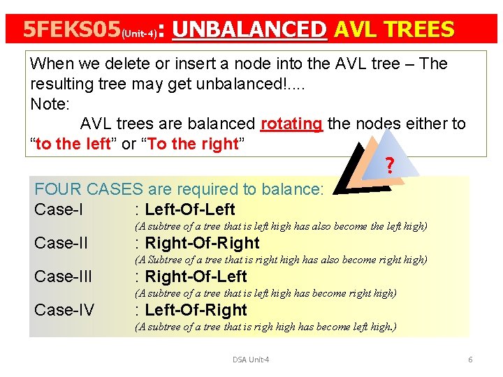
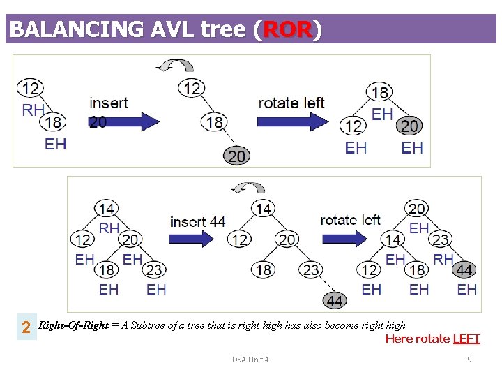
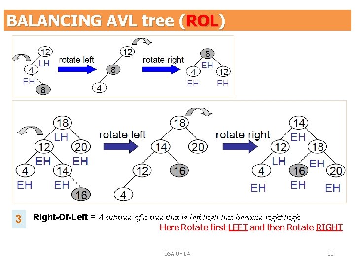
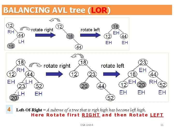
5 FEKS 05(Unit-4): UNBALANCED AVL TREES When we delete or insert a node into the AVL tree – The resulting tree may get unbalanced!. . Note: AVL trees are balanced rotating the nodes either to “to the left” or “To the right” ? FOUR CASES are required to balance: Case-I : Left-Of-Left (A subtree of a tree that is left high has also become the left high) Case-II : Right-Of-Right (A Subtree of a tree that is right high has also become right high) Case-III : Right-Of-Left (A subtree of a tree that is left high has become right high) Case-IV : Left-Of-Right (A subtree of a tree that is righ has become left high. ) DSA Unit-4 6

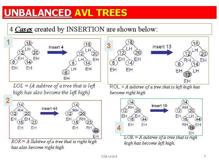
UNBALANCED AVL TREES 4 Cases created by INSERTION are shown below: 1 3 LOL = (A subtree of a tree that is left high has also become the left high) ROL = A subtree of a tree that is left high has become right high 2 4 LOR = A subtree of a tree that is righ has become left high. ROR = A Subtree of a tree that is right high has also become right high DSA Unit-4 7

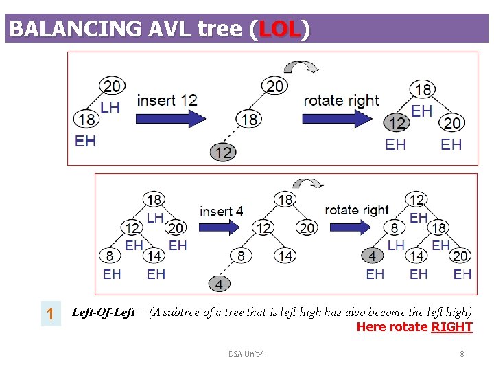
BALANCING AVL tree (LOL) 1 Left-Of-Left = (A subtree of a tree that is left high has also become the left high) Here rotate RIGHT DSA Unit-4 8

BALANCING AVL tree (ROR) 2 Right-Of-Right = A Subtree of a tree that is right high has also become right high Here rotate LEFT DSA Unit-4 9

BALANCING AVL tree (ROL) 3 Right-Of-Left = A subtree of a tree that is left high has become right high Here Rotate first LEFT and then Rotate RIGHT DSA Unit-4 10

BALANCING AVL tree (LOR) 4 Left-Of-Right = A subtree of a tree that is righ has become left high. Here Rotate first RIGHT and then Rotate LEFT DSA Unit-4 11

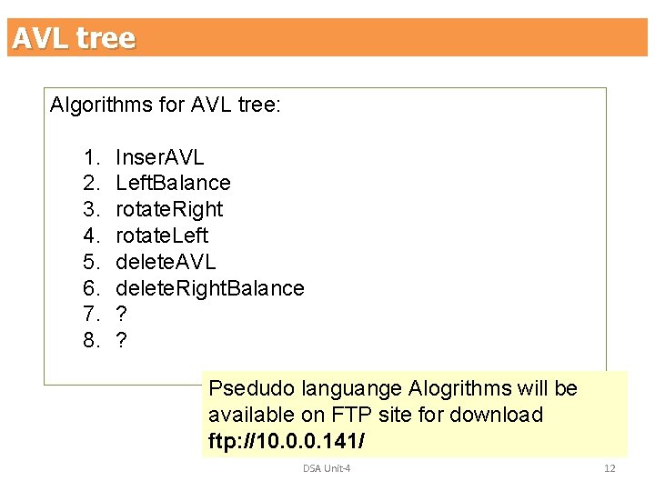
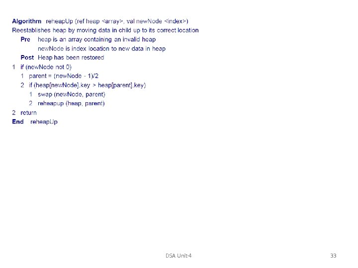
AVL tree Algorithms for AVL tree: 1. 2. 3. 4. 5. 6. 7. 8. Inser. AVL Left. Balance rotate. Right rotate. Left delete. AVL delete. Right. Balance ? ? Psedudo languange Alogrithms will be available on FTP site for download ftp: //10. 0. 0. 141/ DSA Unit-4 12

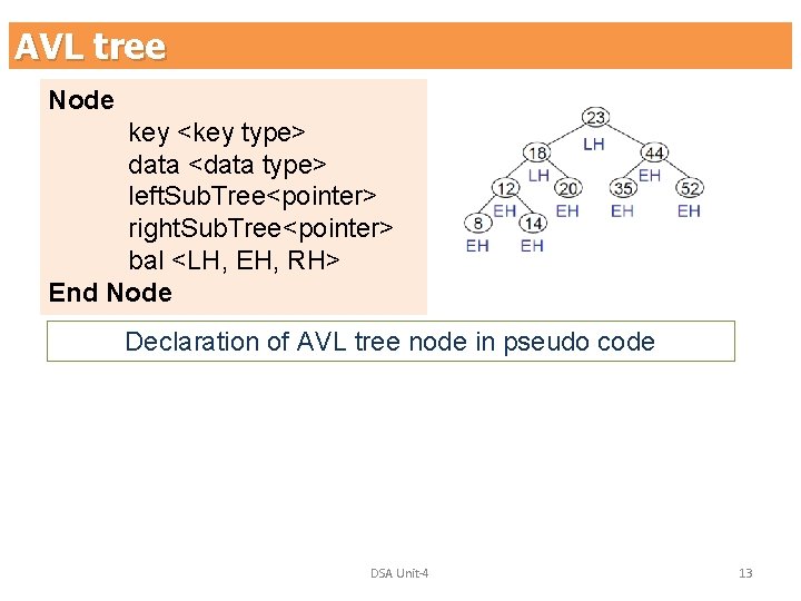
AVL tree Node key <key type> data <data type> left. Sub. Tree<pointer> right. Sub. Tree<pointer> bal <LH, EH, RH> End Node Declaration of AVL tree node in pseudo code DSA Unit-4 13

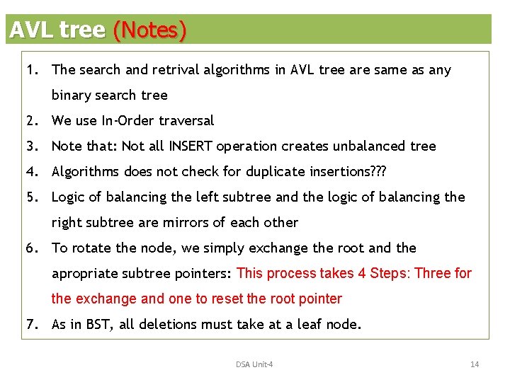
AVL tree (Notes) 1. The search and retrival algorithms in AVL tree are same as any binary search tree 2. We use In-Order traversal 3. Note that: Not all INSERT operation creates unbalanced tree 4. Algorithms does not check for duplicate insertions? ? ? 5. Logic of balancing the left subtree and the logic of balancing the right subtree are mirrors of each other 6. To rotate the node, we simply exchange the root and the apropriate subtree pointers: This process takes 4 Steps: Three for the exchange and one to reset the root pointer 7. As in BST, all deletions must take at a leaf node. DSA Unit-4 14

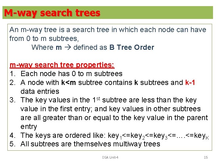
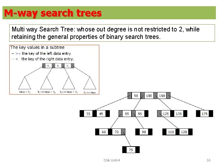
M-way search trees An m-way tree is a search tree in which each node can have from 0 to m subtrees, Where m defined as B Tree Order m-way search tree properties: 1. Each node has 0 to m subtrees 2. A node with k<m subtree contains k subtrees and k-1 data entries 3. The key values in the 1 st subtree are less than the key value in the first entry; and key values in other subtrees are all greater than or equal to the key value in the parent entry 4. The keys are ordered like: key 1<=key 2<=key 3<=…. <=key. K 5. All subtrees are themselves multiway trees DSA Unit-4 15

M-way search trees Multi way Search Tree: whose out degree is not restricted to 2, while retaining the general properties of binary search trees. DSA Unit-4 16

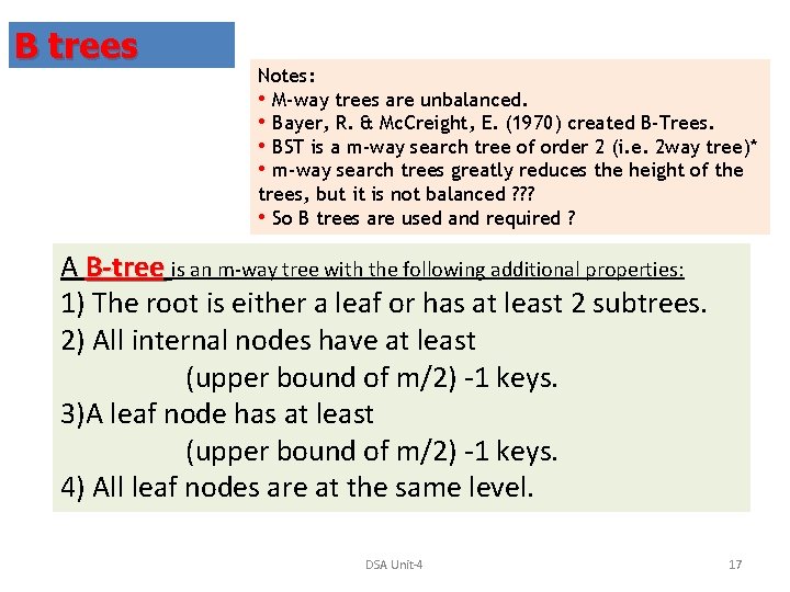
B trees Notes: • M-way trees are unbalanced. • Bayer, R. & Mc. Creight, E. (1970) created B-Trees. • BST is a m-way search tree of order 2 (i. e. 2 way tree)* • m-way search trees greatly reduces the height of the trees, but it is not balanced ? ? ? • So B trees are used and required ? A B-tree is an m-way tree with the following additional properties: 1) The root is either a leaf or has at least 2 subtrees. 2) All internal nodes have at least (upper bound of m/2) -1 keys. 3)A leaf node has at least (upper bound of m/2) -1 keys. 4) All leaf nodes are at the same level. DSA Unit-4 17

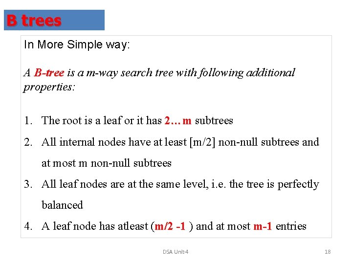
B trees In More Simple way: A B-tree is a m-way search tree with following additional properties: 1. The root is a leaf or it has 2…m subtrees 2. All internal nodes have at least [m/2] non-null subtrees and at most m non-null subtrees 3. All leaf nodes are at the same level, i. e. the tree is perfectly balanced 4. A leaf node has atleast (m/2 -1 ) and at most m-1 entries DSA Unit-4 18

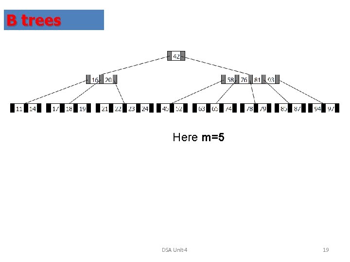
B trees Here m=5 DSA Unit-4 19

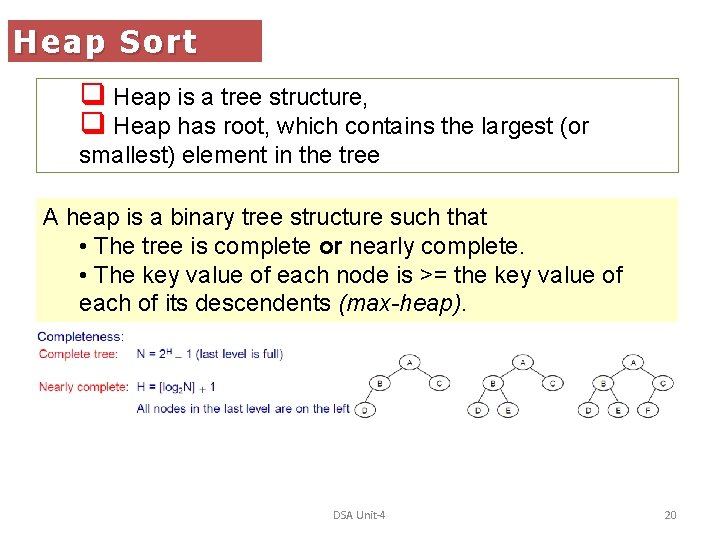
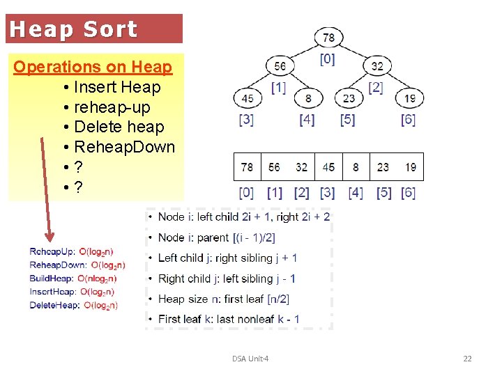
Heap Sort q Heap is a tree structure, q Heap has root, which contains the largest (or smallest) element in the tree A heap is a binary tree structure such that • The tree is complete or nearly complete. • The key value of each node is >= the key value of each of its descendents (max-heap). DSA Unit-4 20

DSA Unit-4 21

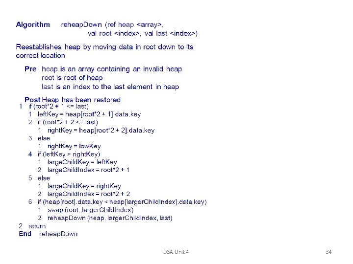
Heap Sort Operations on Heap • Insert Heap • reheap-up • Delete heap • Reheap. Down • ? DSA Unit-4 22

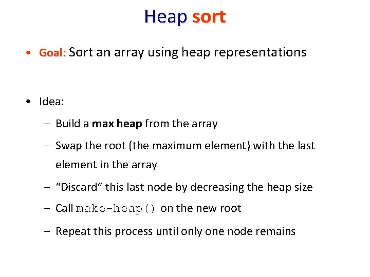
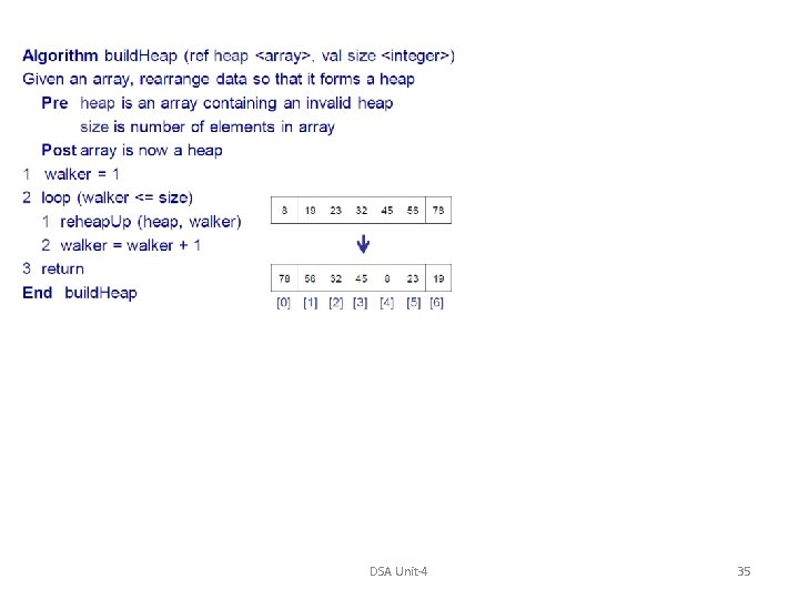
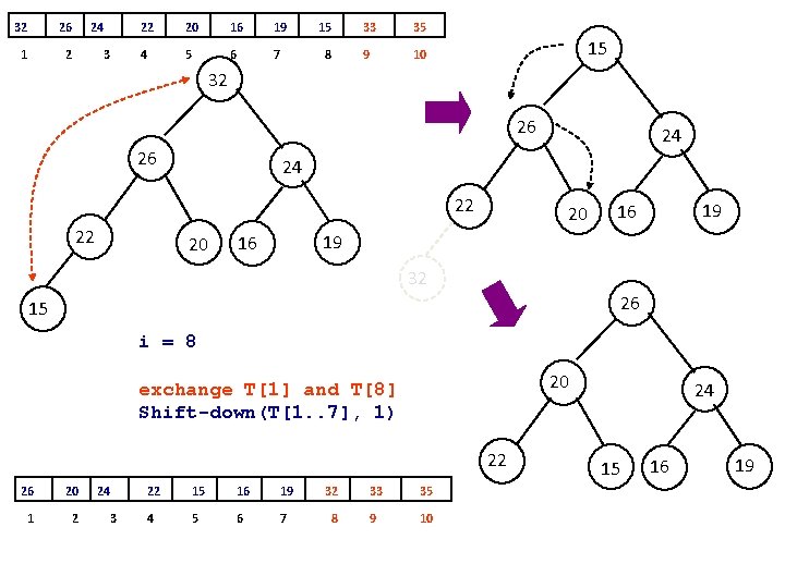
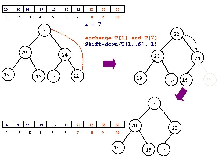
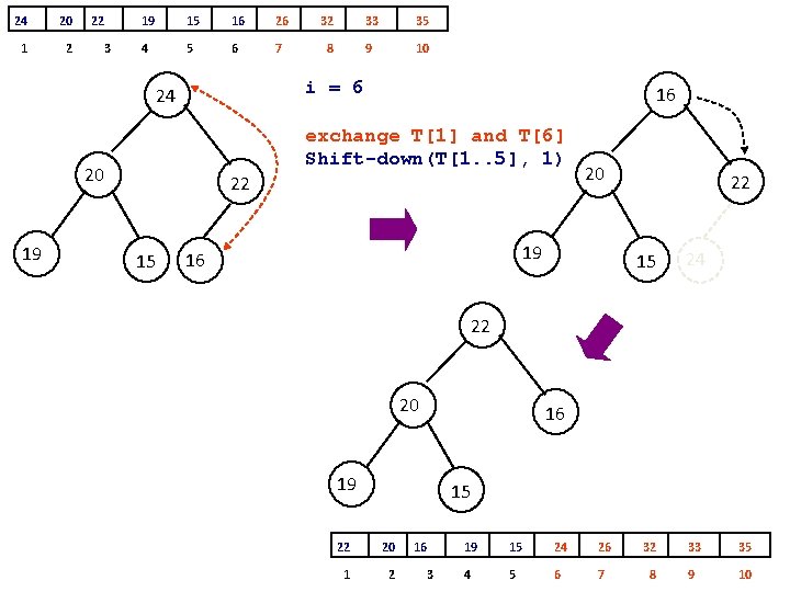
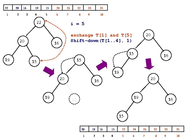
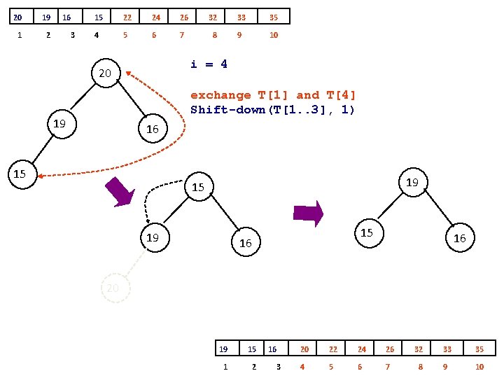
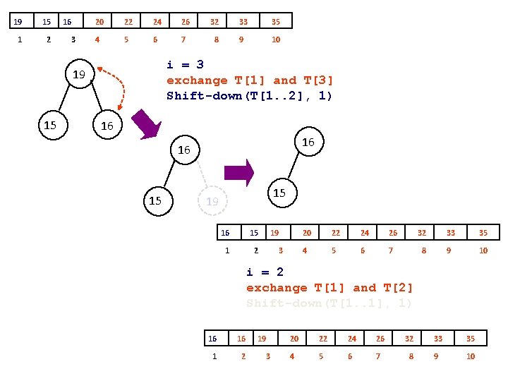
Heap sort • Goal: Sort an array using heap representations • Idea: – Build a max heap from the array – Swap the root (the maximum element) with the last element in the array – “Discard” this last node by decreasing the heap size – Call make-heap() on the new root – Repeat this process until only one node remains
![procedure heapsort T1 n T is an array to be sorted procedure heapsort (T[1. . n]) { T is an array to be sorted }](https://slidetodoc.com/presentation_image_h2/847c1e775db22c5a09cc9ca80daa7644/image-24.jpg)
procedure heapsort (T[1. . n]) { T is an array to be sorted } make-heap(T) for i <- n downto 2 do exchange T[1] and T[i] shift-down(T[1. . i-1], 1) Page# 167 procedure make-heap (T[1. . n]) { This procedure makes the array T[1. . n] into heap } for i <- cel[n/2] downto 1 do shift-down(T, i)
![Page 165 procedure shiftdown T1 n i This procedure shifts node i Page# 165 procedure shift-down (T[1. . n], i) { This procedure shifts node i](https://slidetodoc.com/presentation_image_h2/847c1e775db22c5a09cc9ca80daa7644/image-25.jpg)
Page# 165 procedure shift-down (T[1. . n], i) { This procedure shifts node i down so as to re-establish the heap property in T[1. . n] We suppose that T would be a heap if T[i] were sufficiently large. We also suppose 1 <= i <= n } k <- i repeat j <- k { find the larger child of node j } if 2 j <= n and T[2 j] > T[k] then k <- 2 j if 2 j < n and T[2 j+1] > T[k] then k <- 2 j+1 exchange T[j] and T[k] { if j = k, then the node has arrived at its final position } until j = k

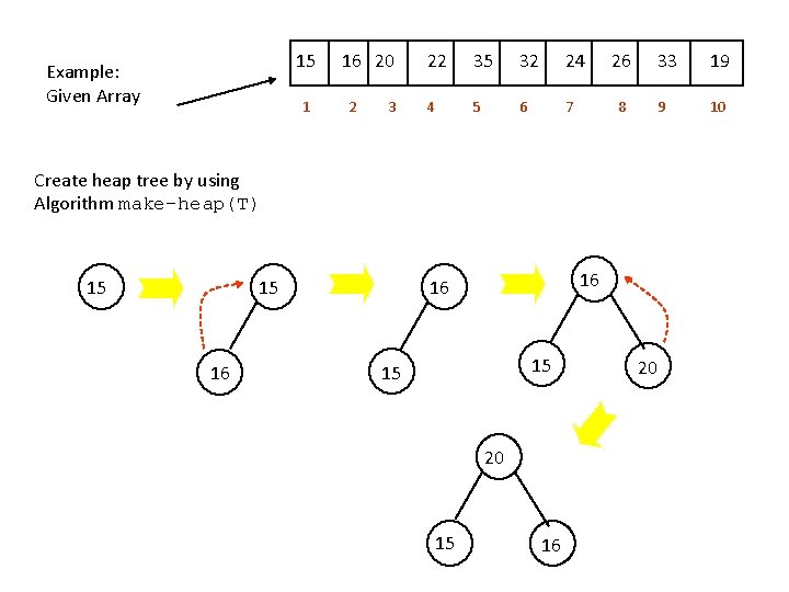
15 Example: Given Array 1 16 20 2 3 22 35 32 24 4 5 6 7 26 8 Create heap tree by using Algorithm make-heap(T) 15 15 16 16 16 15 15 20 15 16 20 33 19 9 10

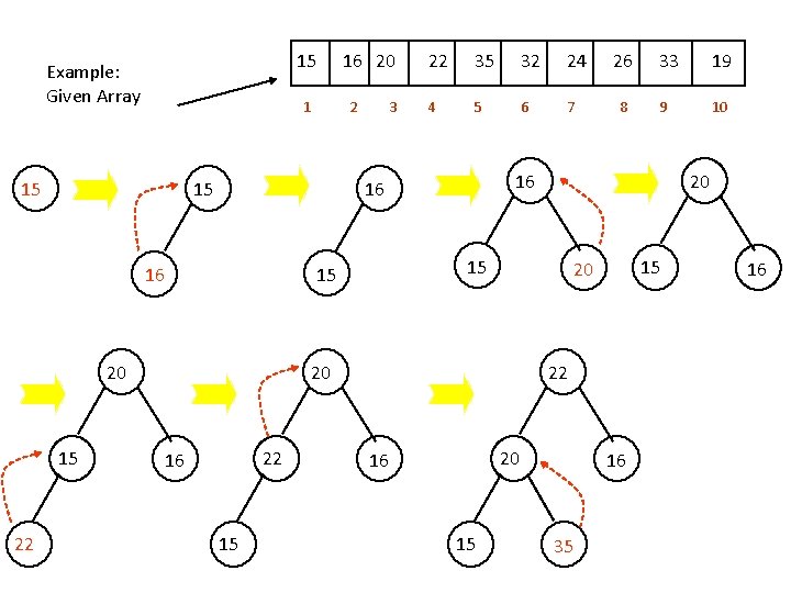
15 Example: Given Array 1 15 3 22 35 32 24 4 5 6 7 20 22 15 19 9 10 15 20 20 16 8 33 20 15 15 26 16 16 16 22 2 15 15 16 20 22 20 16 15 16 35 16

15 Example: Given Array 1 22 20 15 2 3 22 35 32 24 4 5 6 7 22 35 16 15 35 20 22 32 20 16 24 26 8 35 22 16 35 15 16 20 32 33 19 9 10

15 16 1 2 20 3 22 35 32 24 26 33 19 4 5 6 7 8 9 10 35 35 22 22 32 15 24 16 20 35 15 15 20 32 20 16 24 16 35 26 22 26 32 26 24 22 15 32 20 33 16 24

15 16 1 2 20 3 22 35 32 24 26 33 19 4 5 6 7 8 9 10 35 35 26 33 15 33 32 20 26 24 16 15 22 32 22 24 16 20 19 Final build - a heap tree 35 33 1 2 32 3 26 20 16 24 15 22 19 4 5 6 7 8 9 10

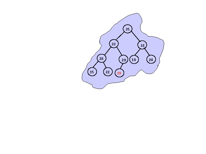
35 33 32 26 15 20 22 19 16 24

Heap Sort 1. The heap sort algorithm is improved version of the “straight-selection sort” 2. Finding the smallest element among the n elements requires n-1 comparisons 3. Heap is a tree structure, we do not need to scan the complete list to locate the largest key/element 4. Because of above property: it makes heap sort much faster than selection sort Homework Q: What is application of Heap Sort technique? DSA Unit-4 32

DSA Unit-4 33

DSA Unit-4 34

DSA Unit-4 35

DSA Unit-4 36

DSA Unit-4 37
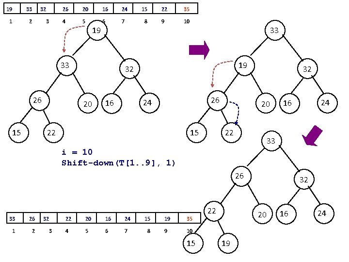
![procedure heapsort T1 n T is an array to be sorted procedure heapsort (T[1. . n]) { T is an array to be sorted }](https://slidetodoc.com/presentation_image_h2/847c1e775db22c5a09cc9ca80daa7644/image-38.jpg)
procedure heapsort (T[1. . n]) { T is an array to be sorted } make-heap(T) for i <- n downto 2 do exchange T[1] and T[i] shift-down(T[1. . i-1], 1) 35 33 32 exchange T[1] and T[i] 26 i = 10 exchange T[1] and T[10] Shift-down(T[1. . 9], 1) 35 33 1 2 32 3 15 20 22 19 26 20 16 24 15 22 19 4 5 6 7 8 9 10 16 24
![procedure heapsort T1 n T is an array to be sorted procedure heapsort (T[1. . n]) { T is an array to be sorted }](https://slidetodoc.com/presentation_image_h2/847c1e775db22c5a09cc9ca80daa7644/image-39.jpg)
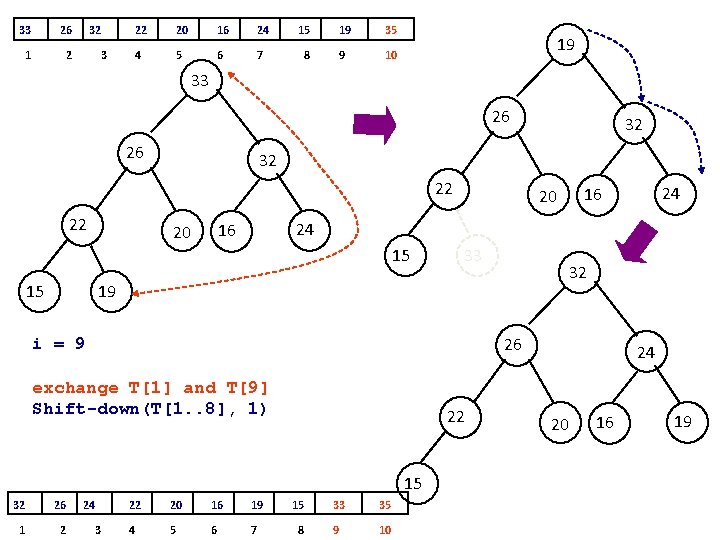
procedure heapsort (T[1. . n]) { T is an array to be sorted } make-heap(T) for i <- n downto 2 do exchange T[1] and T[i] shift-down(T[1. . i-1], 1) 19 33 32 26 20 i = 10 15 Shift-down(T[1. . 9], 1) 19 33 1 2 32 3 22 35 26 20 16 24 15 22 35 4 5 6 7 8 9 10 16 24

19 33 1 2 32 3 26 20 16 24 15 22 35 4 5 6 7 8 9 10 19 33 33 26 15 19 32 20 26 24 16 22 15 32 20 22 24 16 33 i = 10 Shift-down(T[1. . 9], 1) 26 33 26 1 2 32 3 22 20 16 24 15 19 35 4 5 6 7 8 9 10 15 22 32 20 19 16 24

33 26 1 2 32 3 22 20 16 24 15 19 35 4 5 6 7 8 9 10 19 33 26 26 32 22 22 20 15 33 32 19 26 i = 9 exchange T[1] and T[9] Shift-down(T[1. . 8], 1) 22 15 32 26 1 2 24 3 24 16 20 15 32 22 20 16 19 15 33 35 4 5 6 7 8 9 10 24 20 16 19

32 26 1 2 24 3 22 20 16 19 15 33 35 4 5 6 7 8 9 10 15 32 26 26 24 22 22 24 20 20 19 16 32 26 15 i = 8 20 exchange T[1] and T[8] Shift-down(T[1. . 7], 1) 22 26 20 1 2 24 3 22 15 16 19 32 33 35 4 5 6 7 8 9 10 24 15 16 19

26 20 1 2 24 3 19 15 16 22 32 33 35 4 5 6 7 8 9 10 i = 7 26 22 exchange T[1] and T[7] Shift-down(T[1. . 6], 1) 20 24 19 15 20 22 16 24 19 15 24 24 20 1 2 22 3 19 15 16 26 32 33 35 4 5 6 7 8 9 10 19 20 22 15 16 16 26

24 20 1 2 22 3 19 15 16 26 32 33 35 4 5 6 7 8 9 10 i = 6 24 20 19 22 15 16 exchange T[1] and T[6] Shift-down(T[1. . 5], 1) 20 19 16 22 15 24 22 20 16 19 15 22 20 1 2 16 3 19 15 24 26 32 33 35 4 5 6 7 8 9 10

22 20 1 2 16 3 19 15 24 26 32 33 35 4 5 6 7 8 9 10 22 i = 5 20 20 exchange T[1] and T[5] Shift-down(T[1. . 4], 1) 16 15 19 16 15 15 19 20 16 19 22 16 15 20 19 1 2 16 3 15 22 24 26 32 33 35 4 5 6 7 8 9 10

20 19 1 2 16 3 15 22 24 26 32 33 35 4 5 6 7 8 9 10 i = 4 20 exchange T[1] and T[4] Shift-down(T[1. . 3], 1) 19 16 15 19 15 16 16 20 19 15 1 2 16 3 20 22 24 26 32 33 35 4 5 6 7 8 9 10

19 15 1 2 16 3 20 22 24 26 32 33 35 4 5 6 7 8 9 10 i = 3 exchange T[1] and T[3] Shift-down(T[1. . 2], 1) 19 15 16 16 16 15 15 19 16 15 1 2 19 3 20 22 24 26 32 33 35 4 5 6 7 8 9 10 i = 2 exchange T[1] and T[2] Shift-down(T[1. . 1], 1) 16 16 1 2 19 3 20 22 24 26 32 33 35 4 5 6 7 8 9 10