458 Fitting models to data I Sum of

458 Fitting models to data – I (Sum of Squares) Fish 458, Lecture 7

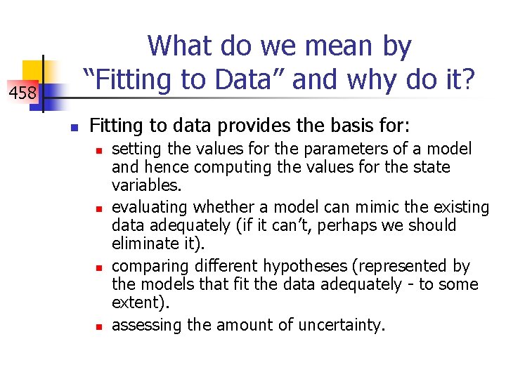
What do we mean by “Fitting to Data” and why do it? 458 n Fitting to data provides the basis for: n n setting the values for the parameters of a model and hence computing the values for the state variables. evaluating whether a model can mimic the existing data adequately (if it can’t, perhaps we should eliminate it). comparing different hypotheses (represented by the models that fit the data adequately - to some extent). assessing the amount of uncertainty.

Keep in Mind 458 n n Models: the parameters, state variables and forcing functions. Data: information we want to use to specify the values for the parameters.

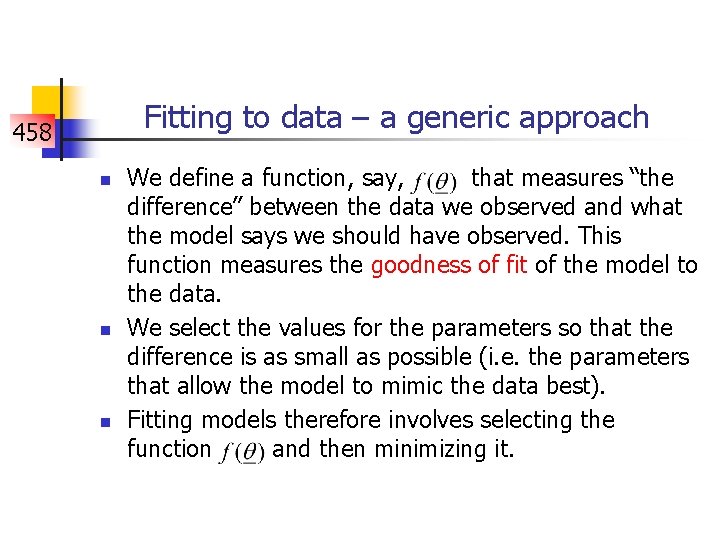
Fitting to data – a generic approach 458 n n n We define a function, say, that measures “the difference” between the data we observed and what the model says we should have observed. This function measures the goodness of fit of the model to the data. We select the values for the parameters so that the difference is as small as possible (i. e. the parameters that allow the model to mimic the data best). Fitting models therefore involves selecting the function and then minimizing it.

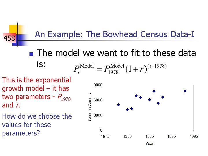
An Example: The Bowhead Census Data-I 458 n The model we want to fit to these data is: This is the exponential growth model – it has two parameters - P 1978 and r. How do we choose the values for these parameters?

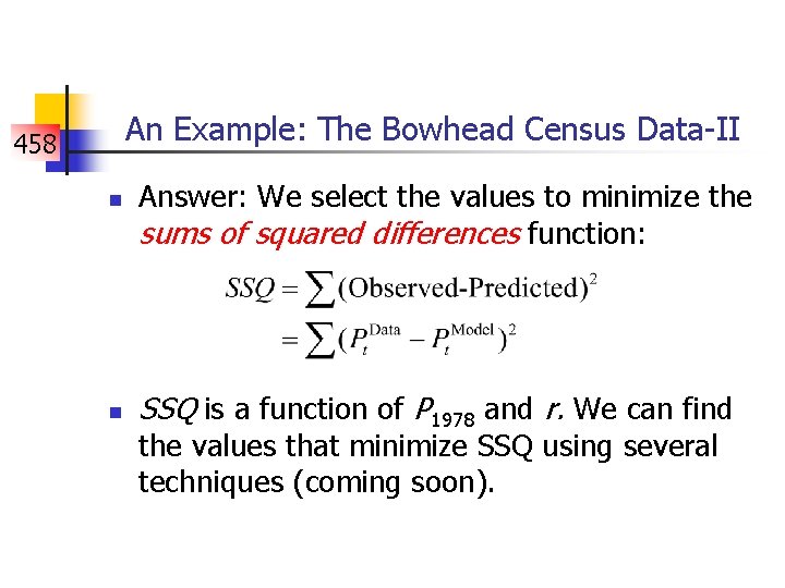
An Example: The Bowhead Census Data-II 458 n n Answer: We select the values to minimize the sums of squared differences function: SSQ is a function of P 1978 and r. We can find the values that minimize SSQ using several techniques (coming soon).

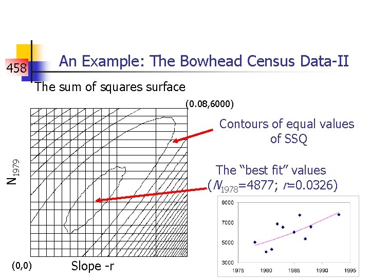
458 An Example: The Bowhead Census Data-II The sum of squares surface (0. 08, 6000) N 1979 Contours of equal values of SSQ (0, 0) The “best fit” values (N 1978=4877; r=0. 0326) Slope -r

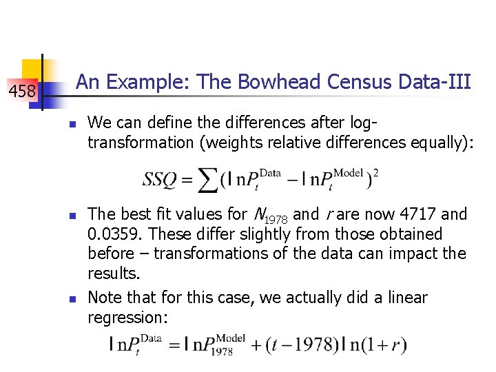
458 An Example: The Bowhead Census Data-III n n n We can define the differences after logtransformation (weights relative differences equally): The best fit values for N 1978 and r are now 4717 and 0. 0359. These differ slightly from those obtained before – transformations of the data can impact the results. Note that for this case, we actually did a linear regression:

458 An Example: The Bowhead Census Data-IV n n To fit the logistic growth model, we just replace the model used to calculate with the logistic model. Transformations: n n n None: equal weight to absolute differences; Log: equal weight to relative differences (i. e. 1 vs 2 weighted equally as 100 vs 200). We often assume a log-transformation because the scale of the data is usually arbitrary.

Computational Methods 458 n n n Direct search (using a sum of squares surface – for 1 -3 parameters). Analytic methods (differentiate SSQ with respect to the parameters and solve the resultant equation – try this for a linear regression). Non-linear optimization methods.

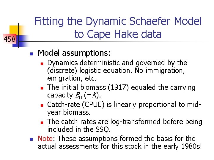
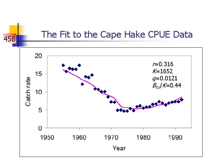
Fitting the Dynamic Schaefer Model to Cape Hake data 458 n Model assumptions: Dynamics deterministic and governed by the (discrete) logistic equation. No immigration, etc. n The initial biomass (1917) equaled the carrying capacity B 0 (=K). n Catch-rate (CPUE) is linearly proportional to midyear biomass. n The catch rates are log-transformed before being included in the SSQ. Note: These assumptions formed the basis for the actual assessments for this stock in the early 1980 s! n n

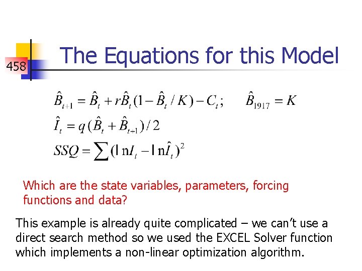
458 The Equations for this Model Which are the state variables, parameters, forcing functions and data? This example is already quite complicated – we can’t use a direct search method so we used the EXCEL Solver function which implements a non-linear optimization algorithm.

458

458 The Fit to the Cape Hake CPUE Data r=0. 316 K=1652 q=0. 0121 B 93/K=0. 44

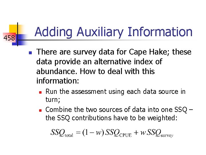
Adding Auxiliary Information 458 n There are survey data for Cape Hake; these data provide an alternative index of abundance. How to deal with this information: n n Run the assessment using each data source in turn; Combine the two sources of data into one SSQ – the SSQ contributions have to be weighted:

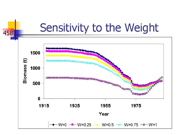
458 Sensitivity to the Weight

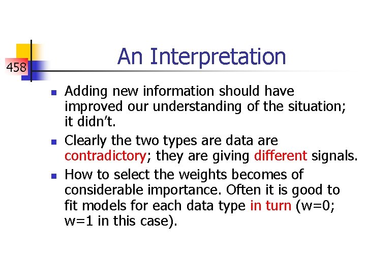
An Interpretation 458 n n n Adding new information should have improved our understanding of the situation; it didn’t. Clearly the two types are data are contradictory; they are giving different signals. How to select the weights becomes of considerable importance. Often it is good to fit models for each data type in turn (w=0; w=1 in this case).

458 Diagnostics This is a case when the sum of squares surface is very complicated and unhelpful 1. Check for patterns in the residuals. 2. Look for influential data points / outliers. 3. Examine sensitivity to changing the data.

Review of Model Fitting-I 458 n n n Identify the questions. Identify the data and the alternative hypotheses. Build a set of alternative models. Select transformations and weightings and build the sum of squares function. Fit the models to the data. Check the diagnostics and reject “unacceptable” models.

Review of Model Fitting - II 458 n Sum of squares allows us to estimate model parameters BUT n How to quantify uncertainty? How to compare models that fit the data “adequately”? n We need Maximum Likelihood methods. n

Readings 458 n n Hilborn and Mangel (1997), Chapter 7 Haddon (2001), Chapter 3