428 XIII Walsh Transform Hadamard Transform 13 A
 13 -A Ideas of Walsh Transforms 8 -point")

![Walsh transform 和 DFT, DCT 有許多相似處 430 , DFT[m, n] = exp( j 2](https://slidetodoc.com/presentation_image_h/d55e614aede2349aba8ac0f8bfa74f4c/image-3.jpg "Walsh transform 和 DFT, DCT 有許多相似處 430 , DFT[m, n] = exp( j 2")
![References for Walsh Transforms 431 [1] K. G. Beanchamp, Walsh Functions and Their Applications,](https://slidetodoc.com/presentation_image_h/d55e614aede2349aba8ac0f8bfa74f4c/image-4.jpg "References for Walsh Transforms 431 [1] K. G. Beanchamp, Walsh Functions and Their Applications,")


 Orthogonal Property (2) Zero-Crossing Property (3) Even / Odd")
 Addition Property 註: Addition modulo 2 (denoted by ) 0 0 =")
![(6) Special functions [n] = 1 when n = 0, [n] = 0 when](https://slidetodoc.com/presentation_image_h/d55e614aede2349aba8ac0f8bfa74f4c/image-14.jpg "(6) Special functions [n] = 1 when n = 0, [n] = 0 when")
![442 (10) Convolution Property If f[n] F[m], g[n] G[m], then h[n] = f[n] g[n]](https://slidetodoc.com/presentation_image_h/d55e614aede2349aba8ac0f8bfa74f4c/image-15.jpg "442 (10) Convolution Property If f[n] F[m], g[n] G[m], then h[n] = f[n] g[n]")
![h[n] = f[n] g[n]= For example, when N = 8, h[3] = f[0]g[3] +](https://slidetodoc.com/presentation_image_h/d55e614aede2349aba8ac0f8bfa74f4c/image-16.jpg "h[n] = f[n] g[n]= For example, when N = 8, h[3] = f[0]g[3] +")
![444 13 -E Butterfly Fast Algorithm (Method 1) John L. Shark’s Algorithm x[0] X[0]](https://slidetodoc.com/presentation_image_h/d55e614aede2349aba8ac0f8bfa74f4c/image-17.jpg "444 13 -E Butterfly Fast Algorithm (Method 1) John L. Shark’s Algorithm x[0] X[0]")
![445 (Method 2) Manz’s Sequence Algorithm x[0] X[0] x[4] -1 x[2] -1 x[1] -1](https://slidetodoc.com/presentation_image_h/d55e614aede2349aba8ac0f8bfa74f4c/image-18.jpg "445 (Method 2) Manz’s Sequence Algorithm x[0] X[0] x[4] -1 x[2] -1 x[1] -1")


![451 H[m, n] 的值 (m = 0, 1, …, 2 k − 1, n](https://slidetodoc.com/presentation_image_h/d55e614aede2349aba8ac0f8bfa74f4c/image-24.jpg "451 H[m, n] 的值 (m = 0, 1, …, 2 k − 1, n")
 Fast (but this advantage is no")


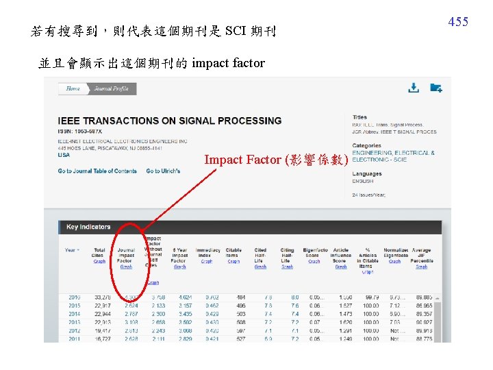
 關於 impact factor (影響係數): 若一個 journal 裡面的文章,被別人引用的次數越多,則這個 journal 的 impact factor 越高")
 要查詢一個領域有哪些 SCI journals 連結至 ISI Web of Knowledge 之後,點選 「Select Category」")

 EI (Engineering Village) 官方網站: www. engineeringvillage. org http: //www. engineeringvillage. com/search/quick. url")
 Conference 排名 Microsoft Academic Search 有列出各領域知名的 conferences 並加以排名 (大致上也是被引用越多的排名越前面) 和通訊與信號處理相關的 conferences,大多排名於 http:")
- Slides: 36
428 XIII. Walsh Transform (Hadamard Transform) 13 -A Ideas of Walsh Transforms 8 -point Walsh transform m 0 1 2 3 4 5 6 7 Advantages of the Walsh transform: (1) Real (2) No multiplication is required (3) Some properties are similar to those of the DFT
Forward and inverse Walsh transforms are similar. forward: , inverse: Alternative names of the Walsh transform: Hadamard transform, Walsh-Hadamard transform Orthogonal Property if m 0 m 1 Zero-Crossing Property Even / Odd Property Fast Algorithm Useful for spectrum analysis Sometimes also useful for implementing the convolution 429
Walsh transform 和 DFT, DCT 有許多相似處 430 , DFT[m, n] = exp( j 2 m n/N),
References for Walsh Transforms 431 [1] K. G. Beanchamp, Walsh Functions and Their Applications, Academic Press, New York, 1975. [2] B. I. Golubov, A. Efimov, and V. Skvortsov, Walsh Series and Transforms: Theory and Applications, Kluwer Academic Publishers, Boston, 1991. [3] H. F. Harmuth, “Applications of Walsh functions in communications, ” IEEE Spectrum, vol. 6, no. 11, pp. 82 -91, Nov. 1969. [4] H. F. Harmuth, Transmission of Information by Orthogonal Functions, Springer-Verlag, New York, 1972.
13 -B Generate the Walsh Transform 2 -point Walsh transform 432 4 -point Walsh transform How do we obtain the 2 k+1 -point Walsh transform from the 2 k-point Walsh transform ? Step 1 Step 2 根據 sign changes 將 rows 的順序重新排列
433 已知 每個 row 的 sign change 數,由上到下分別為 0, 1, 2, 3, …. . , 2 k− 1 則 每個 row 的 sign change 數,由上到下分別為 0, 3, 4, 7, …. . , 2 k+1− 1, 1, 2, 5, 6, …. . , 2 k+1− 2, 若 row 的index 由 0 開始 則 第 n 個 row (n is even and n < N/2) 的 sign change 為 2 n (n is odd and n < N/2) 的 sign change 為 2 n + 1 (n is even and n N/2) 的 sign change 為 2 n+1−N (n is odd and n N/2) 的 sign change 為 2 n−N 要根據 sign change 的數目將 的 row 重新排列
sign changes 0 3 1 2 sign changes 0 3 4 7 1 2 5 6 434
435 Constraint for the number of points of the Walsh transform: N must be a power of 2 (2, 4, 8, 16, 32, ……. . ) Although in Matlab it is possible to define the 12 2 k point or the 20 2 k point Walsh transform, the inverse transform require the floating-point operation.
13 -C Alternative Forms of the Walsh Transform 標準定義 436 from zero-crossing Sequency ordering (i. e. , Walsh ordering) ……. using for signal processing Dyadic ordering (i. e. , Paley ordering) ………. . . using for control Natural ordering (i. e. , Hadamard ordering) ……using for mathematics Sequency ordering Dyadic ordering (Gray Code) Natural ordering (Bit Reversal) W[m, n] row 0 = row 1 = row 2 = row 3 = row 4 = row 5 = row 6 = row 7 = row 0 = row 1 = row 3 = row 2 = row 6 = row 7 = row 5 = row 4 = row 0 = row 4 = row 6 = row 2 = row 3 = row 7 = row 5 = row 1 = [1, 1, 1, 1, 1, 1, 1, 1] [1, 1, 1, 1, 1, 1, 1, 1]
Dyadic ordering Walsh transform Natural ordering Walsh transform 437
binary code to gray code When N = 2 k gk = bk, gq = XOR(bq+1, bq) for q = k 1, k 2, …. , 1 gray code to binary code When N = 2 k bk = gk, bq = XOR(bq+1, gq) for q = k 1, k 2, …. , 1 438
13 -D Properties (1) Orthogonal Property (2) Zero-Crossing Property (3) Even / Odd Property (4) Linear Property If f[n] F[m], g[n] G[m], ( means the Walsh transform) then a f[n] + b g[n] a F[m] + b G[m] 439
440 (5) Addition Property 註: Addition modulo 2 (denoted by ) 0 0 = 1 1 = 0, 0 1 = 1 0 = 1, Example: , therefore 3 7 = 4 : logic addition (similar to XOR)
(6) Special functions [n] = 1 when n = 0, [n] = 0 when n 0 [n] 1, 1 N [n] (7) Shifting property If f[n] F[m], then f[n k] W(k, m) F[m] (8) Modulation property If f[n] F[m], then W(k, n) f[n] F[m k] (9) Parseval’s Theorem If f[n] F[m], g[n] G[m], 441
442 (10) Convolution Property If f[n] F[m], g[n] G[m], then h[n] = f[n] g[n] F[m] G[m] means the “logical convolution” h[n] = f[n] g[n] = 比較: linear convolution circular convolution
h[n] = f[n] g[n]= For example, when N = 8, h[3] = f[0]g[3] + f[1]g[2] + f[2]g[1] + f[3]g[0] + f[4]g[7] + f[5]g[6] + f[6]g[5] + f[7]g[4] h[2] = f[0]g[2] + f[1]g[3] + f[2]g[0] + f[3]g[1] + f[4]g[6] + f[5]g[7] + f[6]g[4] + f[7]g[5] 443
444 13 -E Butterfly Fast Algorithm (Method 1) John L. Shark’s Algorithm x[0] X[0] x[1] -1 x[2] -1 x[4] -1 x[5] -1 x[6] -1 x[7] X[3] -1 x[3] X[7] -1 X[4] X[1] -1 X[2] -1 -1 X[6] -1 -1 X[5]
445 (Method 2) Manz’s Sequence Algorithm x[0] X[0] x[4] -1 x[2] -1 x[1] -1 x[5] -1 x[3] -1 x[7] X[2] -1 x[6] X[1] -1 X[3] X[4] -1 -1 X[5] X[6] -1 X[7] There are other fast implementation algorithm for the Walsh transform.
13 -F Applications 446 Walsh transform 適合作 spectrum analysis,但未必適合作convolution may not be better than DFT, DCT Applications of the Walsh transform Bandwidth reduction High resolution Modulation and Multiplexing Information coding Feature extraction ECG signal (in medical signal processing) analysis Hadamard spectrometer Avoiding quantization error
447 • The Walsh transform is suitable for the function that is a combination of Step functions New Applications: CDMA (code division multiple access)
448 13 -G Jacket Transform 把部分的 1 用 取代 4 -point Jacket transform 2 k+1 -point Jacket P: row permutation [Ref] M. H. Lee, “A new reverse Jacket transform and its fast algorithm, ” IEEE Trans. Circuits Syst. -II , vol. 47, pp. 39 -46, 2000.
449 13 -H Haar Transform N = 2 N = 4 N = 8 [Ref] H. F. Harmuth, Transmission of Information by Orthogonal Functions, Springer-Verlag, New York, 1972
N = 16 450
451 H[m, n] 的值 (m = 0, 1, …, 2 k − 1, n = 0, 1, …, 2 k − 1): H[0, n] = 1 for all n If 2 h m < 2 h+1 H[m, n] = 1 for (m − 2 h)2 k−h n < (m − 2 h +1/2)2 k−h H[m, n] = − 1 for (m − 2 h +1/2)2 k−h n < (m − 2 h +1)2 k−h H[m, n] = 0 otherwise 運算量比 Walsh transforms 更少 Applications: localized spectrum analysis, edge detection Transforms Running Time terms required for NRMSE < 10 5 DFT 9. 5 sec 43 Walsh Transform 2. 2 sec 65 Haar Transform 0. 3 sec 128
452 Main Advantage of the Haar Transform (1) Fast (but this advantage is no longer important) (2) Analysis of the local high frequency component (The wavelet transform is a generalization of the Haar transform) (3) Extracting local features (Example: Adaboost face detection)
附錄十三 SCI Papers 查詢方式 453 我們經常聽到 SCI 論文,impact factor…. 那麼什麼是 SCI 和 impact factor? 什麼樣的論文是 SCI Papers? Impact factor 號如何查詢? SCI 全名: Science Citation Index (A) SCI 相關網站:ISI Web of Knowledge 連結至 ISI Web of Knowledge http: //admin-apps. webofknowledge. com/JCR? RQ=HOME 註:必需要在台大上網,或是在其他有付錢給 ISI 的學術單位上網, 才可以使用 ISI Web of Knowledge
456 (C) 關於 impact factor (影響係數): 若一個 journal 裡面的文章,被別人引用的次數越多,則這個 journal 的 impact factor 越高 一般而言, impact factor 在 2. 5 以上的 journals,已經算是高水準的期刊 Nature 的 impact factor 為 45 Science 的 impact factor 為 40 IEEE 系列的期刊的 impact factors 通常在 2 到 6 之間 IEEE Trans. Image Processing的 impact factors 在 5 左右 IEEE Trans. Signal Processing的 impact factors 在 5 左右 中等水準的期刊的 impact factors 在 1 到 3 之間
457 (D) 要查詢一個領域有哪些 SCI journals 連結至 ISI Web of Knowledge 之後,點選 「Select Category」
458 點選 category 之後再按 submit
459 (E) EI (Engineering Village) 官方網站: www. engineeringvillage. org http: //www. engineeringvillage. com/search/quick. url 查詢期刊或研討會是否為 EI http: //tul. blog. ntu. edu. tw/archives/4627 (F) SSCI (Social Science Citation Index) 比較偏向於社會科學 http: //www. thomsonscientific. com/cgi-bin/jrnlst/jloptions. cgi? PC=J
460 (G) Conference 排名 Microsoft Academic Search 有列出各領域知名的 conferences 並加以排名 (大致上也是被引用越多的排名越前面) 和通訊與信號處理相關的 conferences,大多排名於 http: //academic. research. microsoft. com/Rank. List? entitytype=3&top. Domain. I D=2&sub. Domain. ID=0&last=0&start=1&end=100 或 http: //academic. research. microsoft. com/Rank. List? entitytype=3&top. Domain. I D=8&sub. Domain. ID=0&last=0&start=1&end=100