4 thorder Runge Kutta and the DormandPrince Methods

4 th-order Runge Kutta and the Dormand-Prince Methods Douglas Wilhelm Harder, M. Math. LEL Department of Electrical and Computer Engineering University of Waterloo, Ontario, Canada ece. uwaterloo. ca dwharder@alumni. uwaterloo. ca © 2012 by Douglas Wilhelm Harder. Some rights reserved.

4 th-order Runge Kutta and the Dormand-Prince Methods Outline This topic discusses advanced numerical solutions to initial value problems: – – – Weighted averages and integration techniques Runge-Kutta methods 4 th-order Runge Kutta Adaptive methods The Dormand-Prince method • The Matlab ode 45 function 2

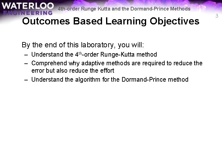
4 th-order Runge Kutta and the Dormand-Prince Methods Outcomes Based Learning Objectives By the end of this laboratory, you will: – Understand the 4 th-order Runge-Kutta method – Comprehend why adaptive methods are required to reduce the error but also reduce the effort – Understand the algorithm for the Dormand-Prince method 3

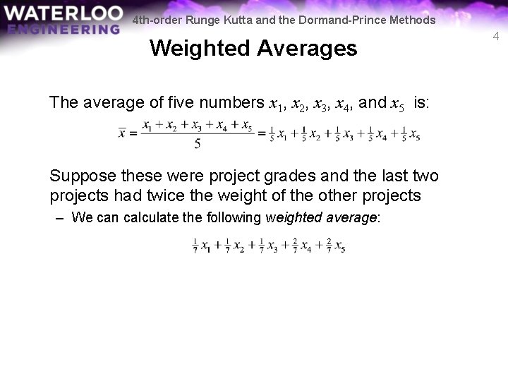
4 th-order Runge Kutta and the Dormand-Prince Methods Weighted Averages The average of five numbers x 1, x 2, x 3, x 4, and x 5 is: Suppose these were project grades and the last two projects had twice the weight of the other projects – We can calculate the following weighted average: 4

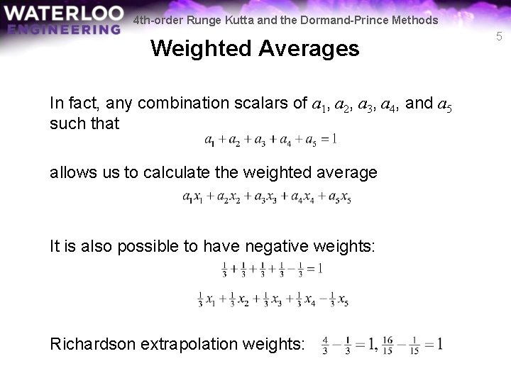
4 th-order Runge Kutta and the Dormand-Prince Methods Weighted Averages In fact, any combination scalars of a 1, a 2, a 3, a 4, and a 5 such that allows us to calculate the weighted average It is also possible to have negative weights: Richardson extrapolation weights: 5

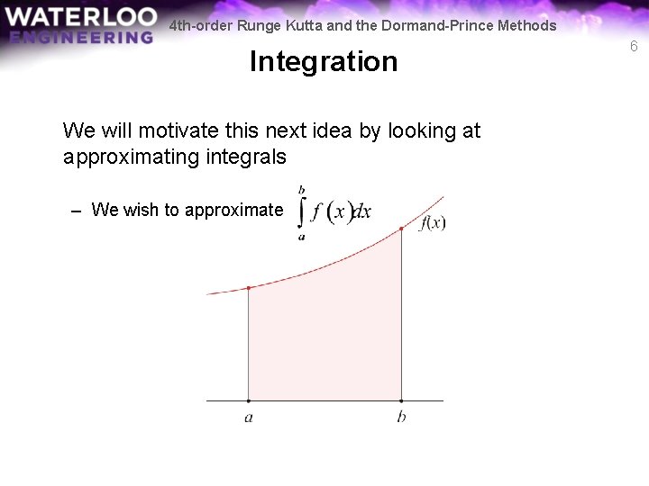
4 th-order Runge Kutta and the Dormand-Prince Methods Integration We will motivate this next idea by looking at approximating integrals – We wish to approximate 6

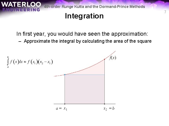
4 th-order Runge Kutta and the Dormand-Prince Methods 7 Integration In first year, you would have seen the approximation: – Approximate the integral by calculating the area of the square a= =b

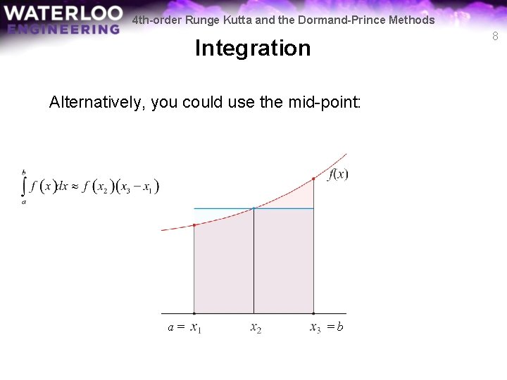
4 th-order Runge Kutta and the Dormand-Prince Methods 8 Integration Alternatively, you could use the mid-point: a= =b

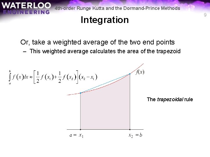
4 th-order Runge Kutta and the Dormand-Prince Methods 9 Integration Or, take a weighted average of the two end points – This weighted average calculates the area of the trapezoid The trapezoidal rule a= =b

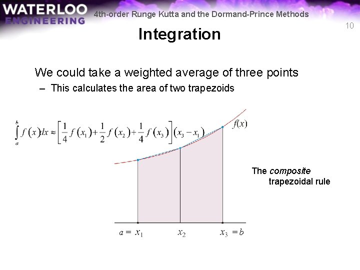
4 th-order Runge Kutta and the Dormand-Prince Methods 10 Integration We could take a weighted average of three points – This calculates the area of two trapezoids The composite trapezoidal rule a= =b

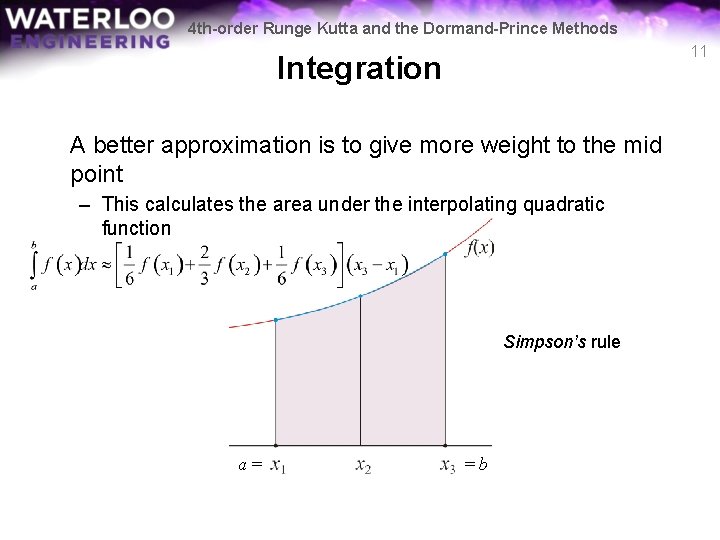
4 th-order Runge Kutta and the Dormand-Prince Methods 11 Integration A better approximation is to give more weight to the mid point – This calculates the area under the interpolating quadratic function Simpson’s rule a= =b

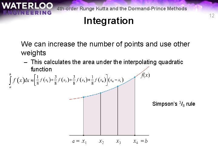
4 th-order Runge Kutta and the Dormand-Prince Methods 12 Integration We can increase the number of points and use other weights – This calculates the area under the interpolating quadratic function Simpson’s 3/8 rule a= =b

4 th-order Runge Kutta and the Dormand-Prince Methods Initial-value Problems We will use the same weighted average idea to find better approximations of an initial-value problem In the last laboratory, we saw – Euler’s method – Heun’s method In this laboratory, we will see: – The 4 th-order Runge Kutta method – The Dormand-Prince method Both use weighted averages 13

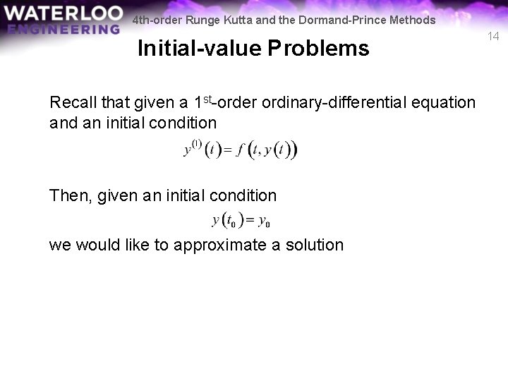
4 th-order Runge Kutta and the Dormand-Prince Methods Initial-value Problems Recall that given a 1 st-order ordinary-differential equation and an initial condition Then, given an initial condition we would like to approximate a solution 14

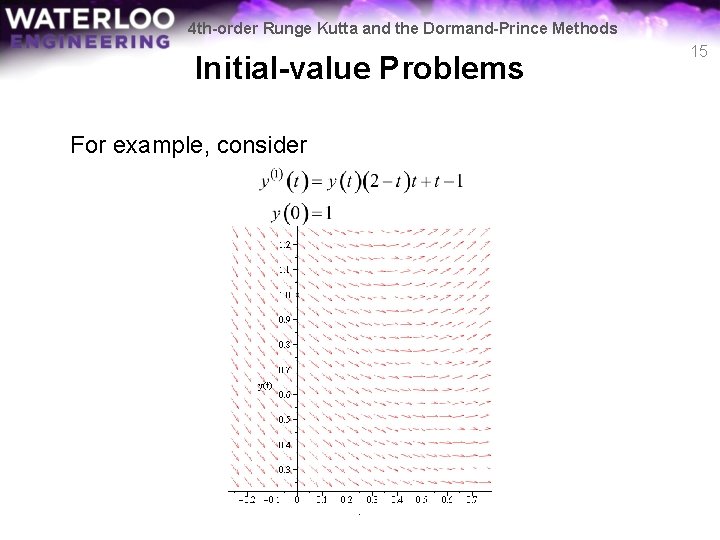
4 th-order Runge Kutta and the Dormand-Prince Methods Initial-value Problems For example, consider 15

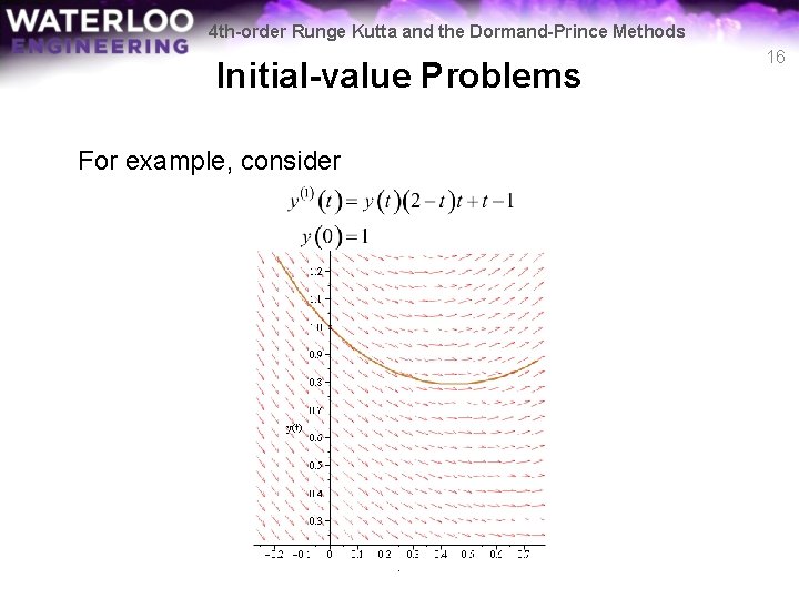
4 th-order Runge Kutta and the Dormand-Prince Methods Initial-value Problems For example, consider 16

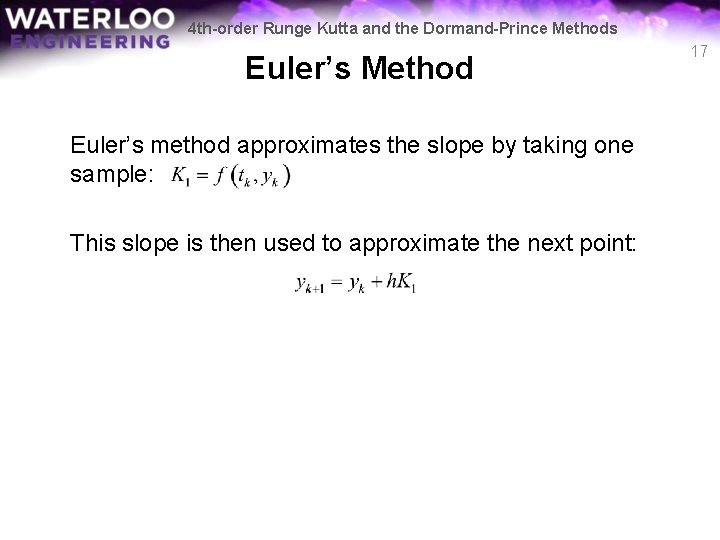
4 th-order Runge Kutta and the Dormand-Prince Methods Euler’s Method Euler’s method approximates the slope by taking one sample: This slope is then used to approximate the next point: 17

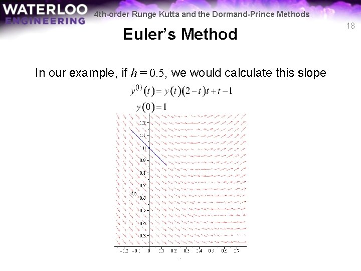
4 th-order Runge Kutta and the Dormand-Prince Methods Euler’s Method In our example, if h = 0. 5, we would calculate this slope 18

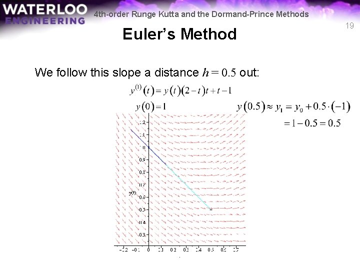
4 th-order Runge Kutta and the Dormand-Prince Methods Euler’s Method We follow this slope a distance h = 0. 5 out: 19

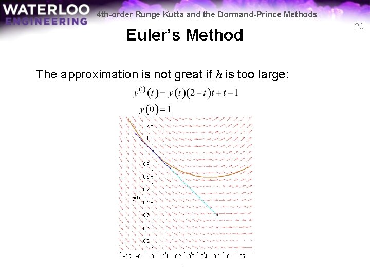
4 th-order Runge Kutta and the Dormand-Prince Methods Euler’s Method The approximation is not great if h is too large: 20

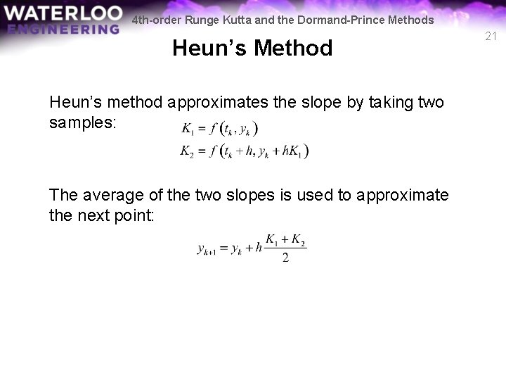
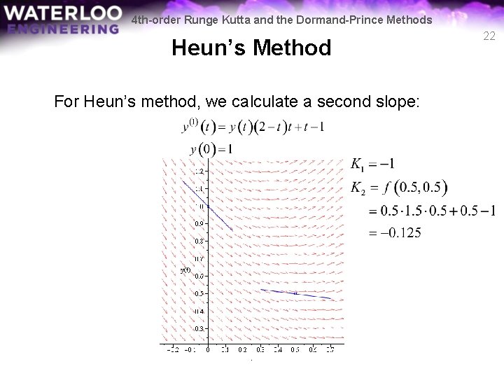
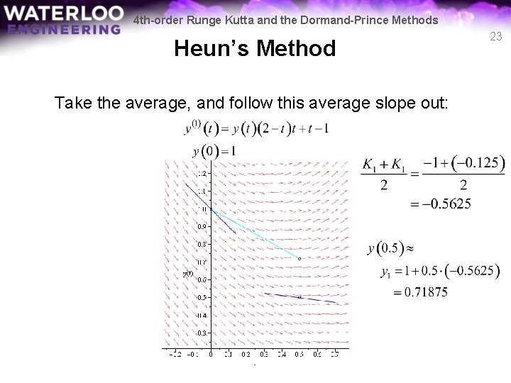
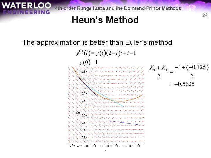
4 th-order Runge Kutta and the Dormand-Prince Methods Heun’s Method Heun’s method approximates the slope by taking two samples: The average of the two slopes is used to approximate the next point: 21

4 th-order Runge Kutta and the Dormand-Prince Methods Heun’s Method For Heun’s method, we calculate a second slope: 22

4 th-order Runge Kutta and the Dormand-Prince Methods Heun’s Method Take the average, and follow this average slope out: 23

4 th-order Runge Kutta and the Dormand-Prince Methods Heun’s Method The approximation is better than Euler’s method 24

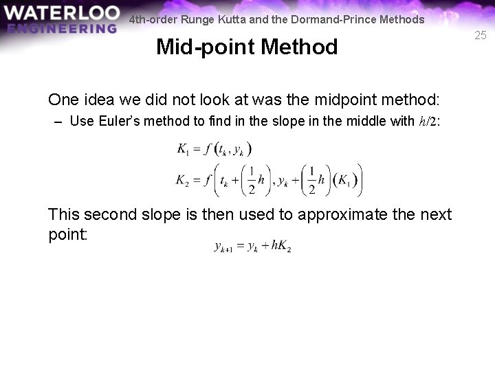
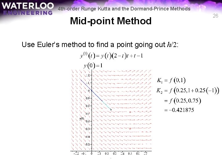
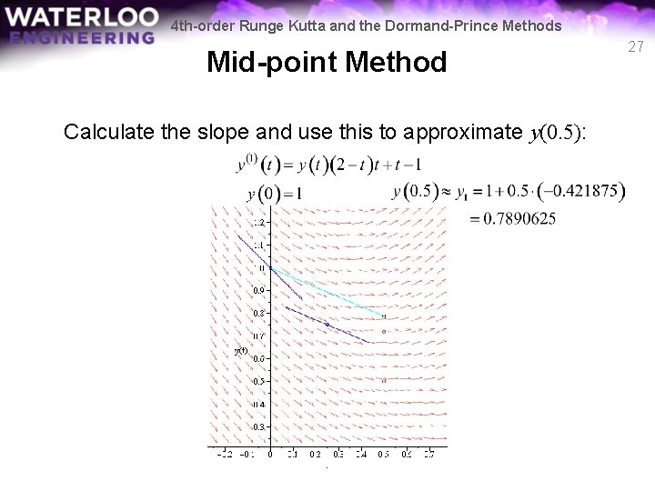
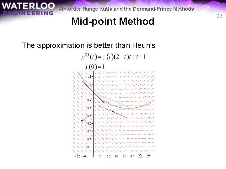
4 th-order Runge Kutta and the Dormand-Prince Methods Mid-point Method One idea we did not look at was the midpoint method: – Use Euler’s method to find in the slope in the middle with h/2: This second slope is then used to approximate the next point: 25

4 th-order Runge Kutta and the Dormand-Prince Methods Mid-point Method Use Euler’s method to find a point going out h/2: 26

4 th-order Runge Kutta and the Dormand-Prince Methods Mid-point Method Calculate the slope and use this to approximate y(0. 5): 27

4 th-order Runge Kutta and the Dormand-Prince Methods Mid-point Method The approximation is better than Heun’s 28

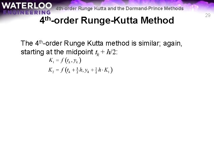
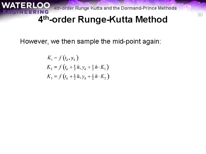
4 th-order Runge Kutta and the Dormand-Prince Methods 4 th-order Runge-Kutta Method The 4 th-order Runge Kutta method is similar; again, starting at the midpoint tk + h/2: 29

4 th-order Runge Kutta and the Dormand-Prince Methods 4 th-order Runge-Kutta Method However, we then sample the mid-point again: 30

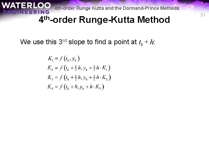
4 th-order Runge Kutta and the Dormand-Prince Methods 4 th-order Runge-Kutta Method We use this 3 rd slope to find a point at tk + h: 31

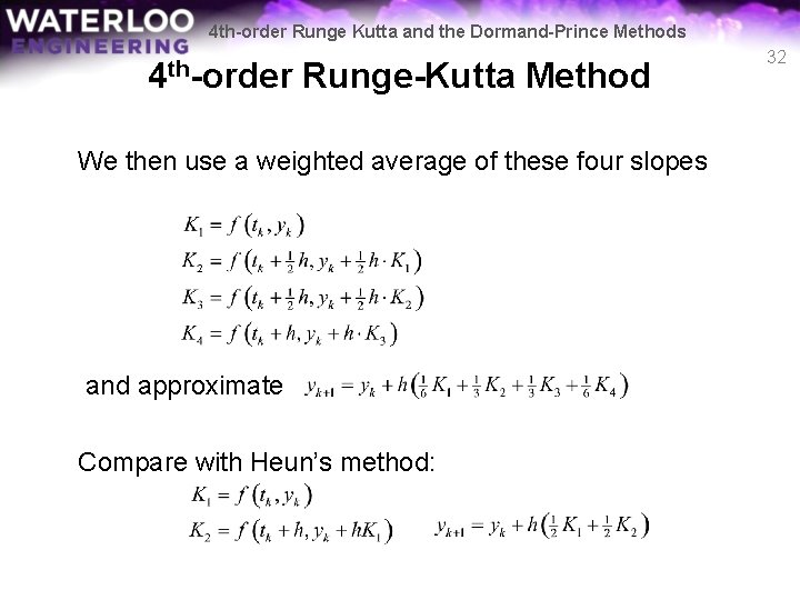
4 th-order Runge Kutta and the Dormand-Prince Methods 4 th-order Runge-Kutta Method We then use a weighted average of these four slopes and approximate Compare with Heun’s method: 32

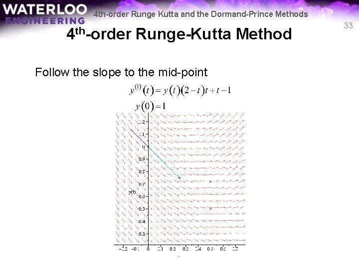
4 th-order Runge Kutta and the Dormand-Prince Methods 4 th-order Runge-Kutta Method Follow the slope to the mid-point 33

4 th-order Runge Kutta and the Dormand-Prince Methods 4 th-order Runge-Kutta Method Determine this slope, K 2: 34

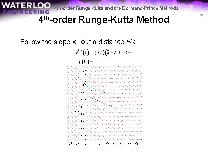
4 th-order Runge Kutta and the Dormand-Prince Methods 4 th-order Runge-Kutta Method Follow the slope K 2 out a distance h/2: 35

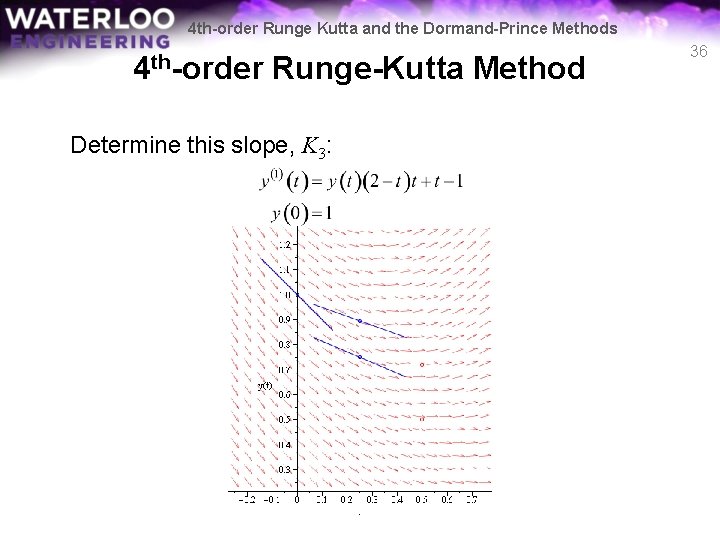
4 th-order Runge Kutta and the Dormand-Prince Methods 4 th-order Runge-Kutta Method Determine this slope, K 3: 36

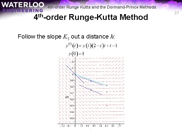
4 th-order Runge Kutta and the Dormand-Prince Methods 4 th-order Runge-Kutta Method Follow the slope K 3 out a distance h: 37

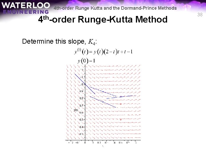
4 th-order Runge Kutta and the Dormand-Prince Methods 4 th-order Runge-Kutta Method Determine this slope, K 4: 38

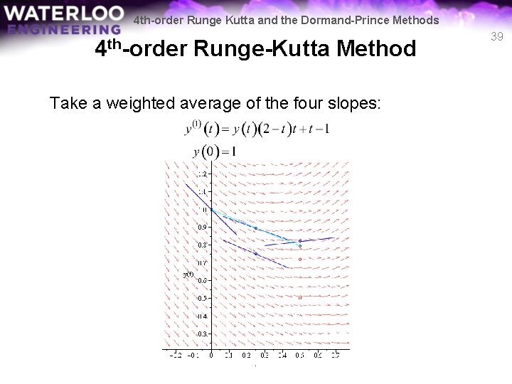
4 th-order Runge Kutta and the Dormand-Prince Methods 4 th-order Runge-Kutta Method Take a weighted average of the four slopes: 39

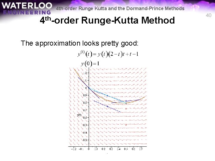
4 th-order Runge Kutta and the Dormand-Prince Methods 4 th-order Runge-Kutta Method The approximation looks pretty good: 40

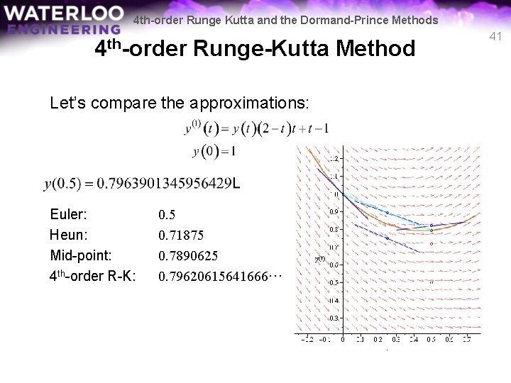
4 th-order Runge Kutta and the Dormand-Prince Methods 4 th-order Runge-Kutta Method Let’s compare the approximations: Euler: Heun: Mid-point: 4 th-order R-K: 0. 5 0. 71875 0. 7890625 0. 79620615641666··· 41

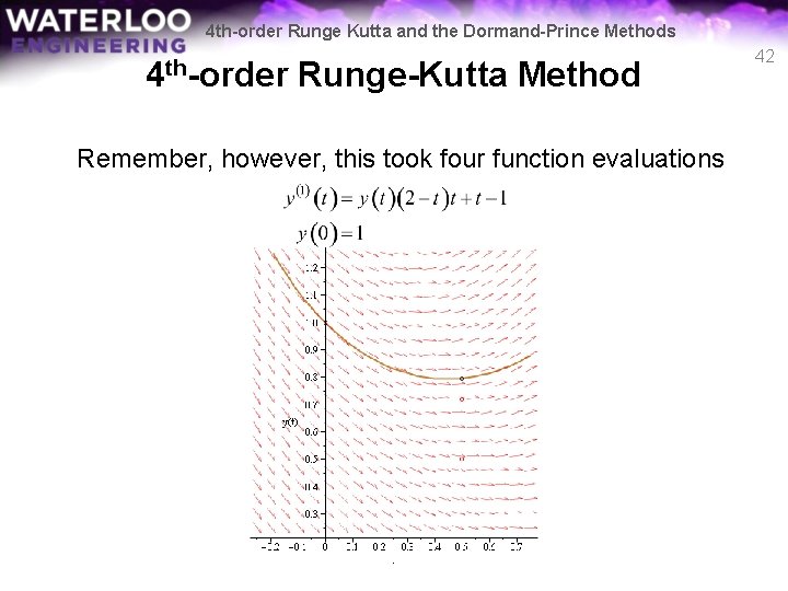
4 th-order Runge Kutta and the Dormand-Prince Methods 4 th-order Runge-Kutta Method Remember, however, this took four function evaluations 42

4 th-order Runge Kutta and the Dormand-Prince Methods 4 th-order Runge-Kutta Method Four steps of Euler’s method is about as good as Heun’s 43

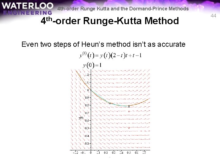
4 th-order Runge Kutta and the Dormand-Prince Methods 4 th-order Runge-Kutta Method Even two steps of Heun’s method isn’t as accurate 44

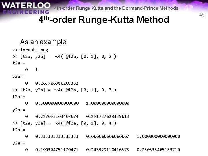
4 th-order Runge Kutta and the Dormand-Prince Methods 4 th-order Runge-Kutta Method As an example, >> format long >> [t 2 a, y 2 a] = rk 4( @f 2 a, [0, 1], 0, 2 ) t 2 a = 0 1 y 2 a = 0 0. 265706380208333 >> [t 2 a, y 2 a] = rk 4( @f 2 a, [0, 1], 0, 3 ) t 2 a = 0 0. 50000000 1. 00000000 y 2 a = 0 0. 227653163407674 0. 251787629335613 >> [t 2 a, y 2 a] = rk 4( @f 2 a, [0, 1], 0, 4 ) t 2 a = 0 0. 33333333 0. 66666667 y 2 a = 0 0. 190364751129471 0. 243328110416578 1. 00000000 0. 250335465183716 45

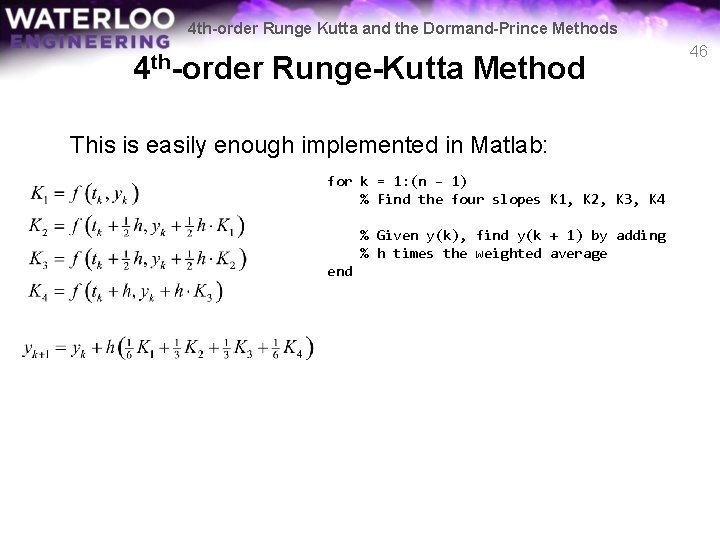
4 th-order Runge Kutta and the Dormand-Prince Methods 4 th-order Runge-Kutta Method This is easily enough implemented in Matlab: for k = 1: (n – 1) % Find the four slopes K 1, K 2, K 3, K 4 % Given y(k), find y(k + 1) by adding % h times the weighted average end 46

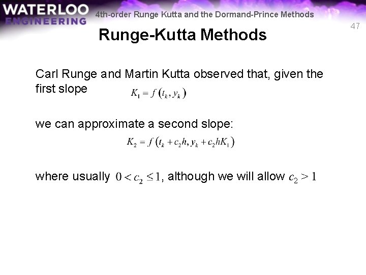
4 th-order Runge Kutta and the Dormand-Prince Methods Runge-Kutta Methods Carl Runge and Martin Kutta observed that, given the first slope we can approximate a second slope: where usually , although we will allow c 2 > 1 47

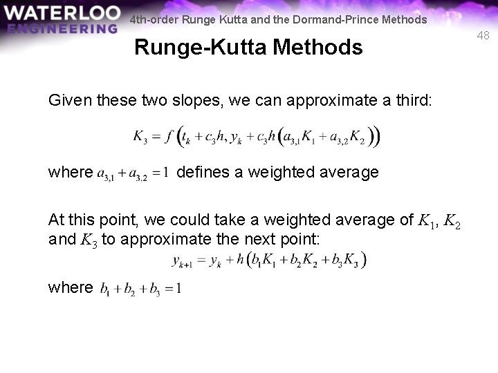
4 th-order Runge Kutta and the Dormand-Prince Methods Runge-Kutta Methods Given these two slopes, we can approximate a third: where defines a weighted average At this point, we could take a weighted average of K 1, K 2 and K 3 to approximate the next point: where 48

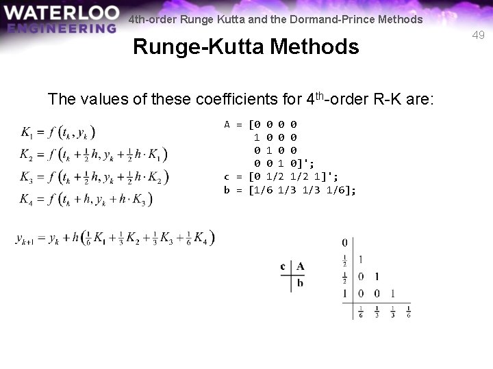
4 th-order Runge Kutta and the Dormand-Prince Methods Runge-Kutta Methods The values of these coefficients for 4 th-order R-K are: A = [0 0 0 0 1 0]'; c = [0 1/2 1]'; b = [1/6 1/3 1/6]; 49

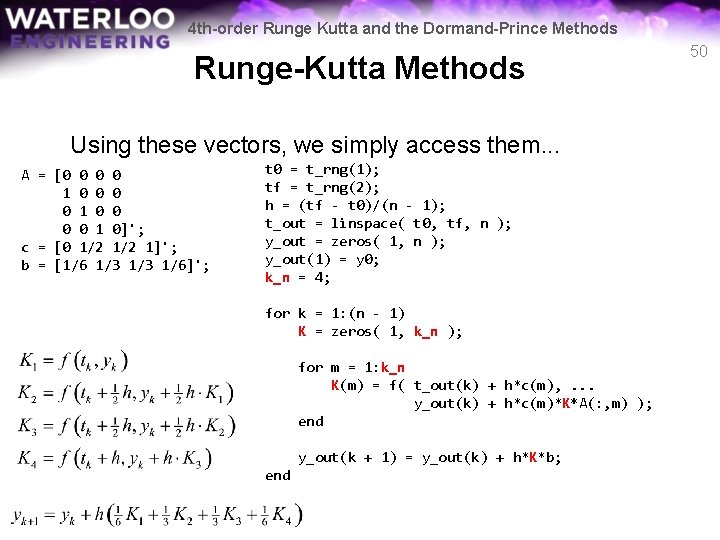
4 th-order Runge Kutta and the Dormand-Prince Methods Runge-Kutta Methods Using these vectors, we simply access them. . . A = [0 0 0 0 1 0]'; c = [0 1/2 1]'; b = [1/6 1/3 1/6]'; t 0 = t_rng(1); tf = t_rng(2); h = (tf - t 0)/(n - 1); t_out = linspace( t 0, tf, n ); y_out = zeros( 1, n ); y_out(1) = y 0; k_n = 4; for k = 1: (n - 1) K = zeros( 1, k_n ); for m = 1: k_n K(m) = f( t_out(k) + h*c(m), . . . y_out(k) + h*c(m)*K*A(: , m) ); end y_out(k + 1) = y_out(k) + h*K*b; end 50

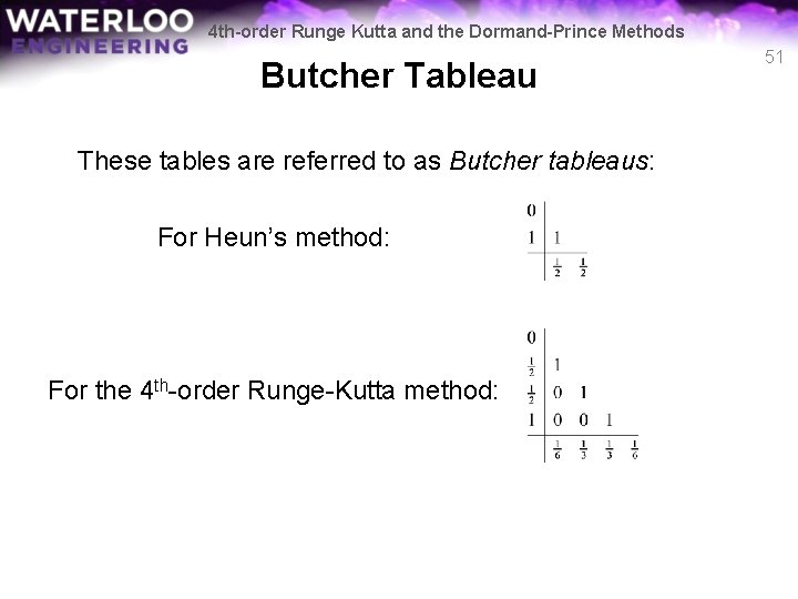
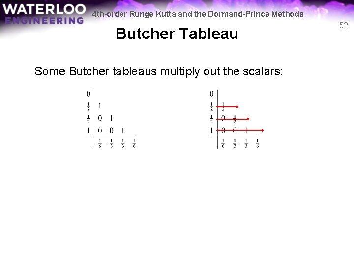
4 th-order Runge Kutta and the Dormand-Prince Methods Butcher Tableau These tables are referred to as Butcher tableaus: For Heun’s method: For the 4 th-order Runge-Kutta method: 51

4 th-order Runge Kutta and the Dormand-Prince Methods Butcher Tableau Some Butcher tableaus multiply out the scalars: 52

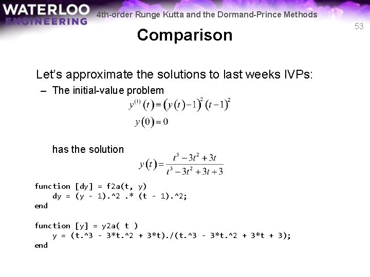
4 th-order Runge Kutta and the Dormand-Prince Methods Comparison Let’s approximate the solutions to last weeks IVPs: – The initial-value problem has the solution function [dy] = f 2 a(t, y) dy = (y - 1). ^2. * (t - 1). ^2; end function [y] = y 2 a( t ) y = (t. ^3 - 3*t. ^2 + 3*t). /(t. ^3 - 3*t. ^2 + 3*t + 3); end 53

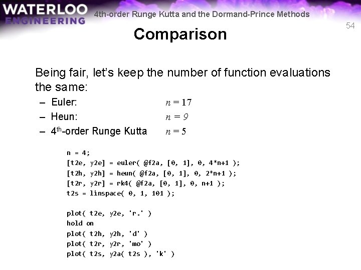
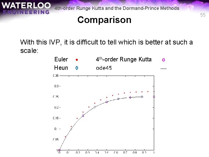
4 th-order Runge Kutta and the Dormand-Prince Methods Comparison Being fair, let’s keep the number of function evaluations the same: – Euler: – Heun: – 4 th-order Runge Kutta n = 17 n=9 n=5 n = 4; [t 2 e, y 2 e] = euler( @f 2 a, [0, 1], 0, 4*n+1 ); [t 2 h, y 2 h] = heun( @f 2 a, [0, 1], 0, 2*n+1 ); [t 2 r, y 2 r] = rk 4( @f 2 a, [0, 1], 0, n+1 ); t 2 s = linspace( 0, 1, 101 ); plot( t 2 e, hold on plot( t 2 h, plot( t 2 r, plot( t 2 s, y 2 e, 'r. ' ) y 2 h, 'd' ) y 2 r, 'mo' ) y 2 a( t 2 s ), 'k' ) 54

4 th-order Runge Kutta and the Dormand-Prince Methods 55 Comparison With this IVP, it is difficult to tell which is better at such a scale: Euler Heun • ◊ 4 th-order Runge Kutta ode 45 o ___

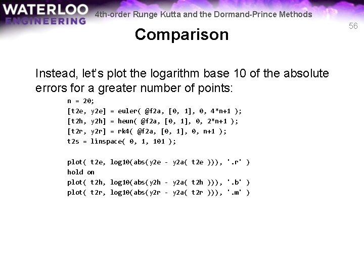
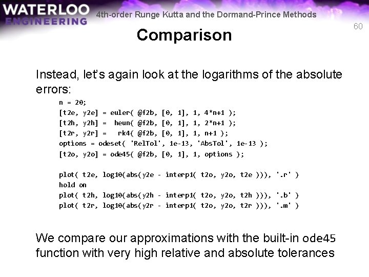
4 th-order Runge Kutta and the Dormand-Prince Methods Comparison Instead, let’s plot the logarithm base 10 of the absolute errors for a greater number of points: n = 20; [t 2 e, y 2 e] = euler( @f 2 a, [0, 1], 0, 4*n+1 ); [t 2 h, y 2 h] = heun( @f 2 a, [0, 1], 0, 2*n+1 ); [t 2 r, y 2 r] = rk 4( @f 2 a, [0, 1], 0, n+1 ); t 2 s = linspace( 0, 1, 101 ); plot( t 2 e, log 10(abs(y 2 e - y 2 a( t 2 e ))), '. r' ) hold on plot( t 2 h, log 10(abs(y 2 h - y 2 a( t 2 h ))), '. b' ) plot( t 2 r, log 10(abs(y 2 r - y 2 a( t 2 r ))), '. m' ) 56

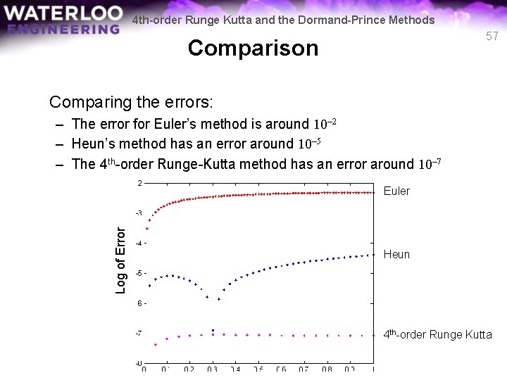
4 th-order Runge Kutta and the Dormand-Prince Methods 57 Comparison Comparing the errors: – The error for Euler’s method is around 10– 2 – Heun’s method has an error around 10– 5 – The 4 th-order Runge-Kutta method has an error around 10– 7 Log of Error Euler Heun 4 th-order Runge Kutta

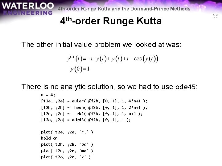
4 th-order Runge Kutta and the Dormand-Prince Methods 4 th-order Runge Kutta The other initial value problem we looked at was: There is no analytic solution, so we had to use ode 45: n = 4; [t 2 e, y 2 e] [t 2 h, y 2 h] [t 2 r, y 2 r] [t 2 o, y 2 o] plot( t 2 e, hold on plot( t 2 h, plot( t 2 r, plot( t 2 o, = euler( @f 2 b, [0, 1], = heun( @f 2 b, [0, 1], = rk 4( @f 2 b, [0, 1], = ode 45( @f 2 b, [0, 1], y 2 e, 'r. ' ) y 2 h, 'bd' ) y 2 r, 'mo' ) y 2 o, 'k' ) 1, 4*n+1 ); 1, 2*n+1 ); 1, n+1 ); 58

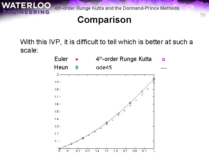
4 th-order Runge Kutta and the Dormand-Prince Methods 59 Comparison With this IVP, it is difficult to tell which is better at such a scale: Euler Heun • ◊ 4 th-order Runge Kutta ode 45 o ___

4 th-order Runge Kutta and the Dormand-Prince Methods Comparison Instead, let’s again look at the logarithms of the absolute errors: n = 20; [t 2 e, y 2 e] = euler( @f 2 b, [0, 1], 1, 4*n+1 ); [t 2 h, y 2 h] = heun( @f 2 b, [0, 1], 1, 2*n+1 ); [t 2 r, y 2 r] = rk 4( @f 2 b, [0, 1], 1, n+1 ); options = odeset( 'Rel. Tol', 1 e-13, 'Abs. Tol', 1 e-13 ); [t 2 o, y 2 o] = ode 45( @f 2 b, [0, 1], 1, options ); plot( t 2 e, log 10(abs(y 2 e - interp 1( t 2 o, y 2 o, t 2 e ))), '. r' ) hold on plot( t 2 h, log 10(abs(y 2 h - interp 1( t 2 o, y 2 o, t 2 h ))), '. b' ) plot( t 2 r, log 10(abs(y 2 r - interp 1( t 2 o, y 2 o, t 2 r ))), '. m' ) We compare our approximations with the built-in ode 45 function with very high relative and absolute tolerances 60

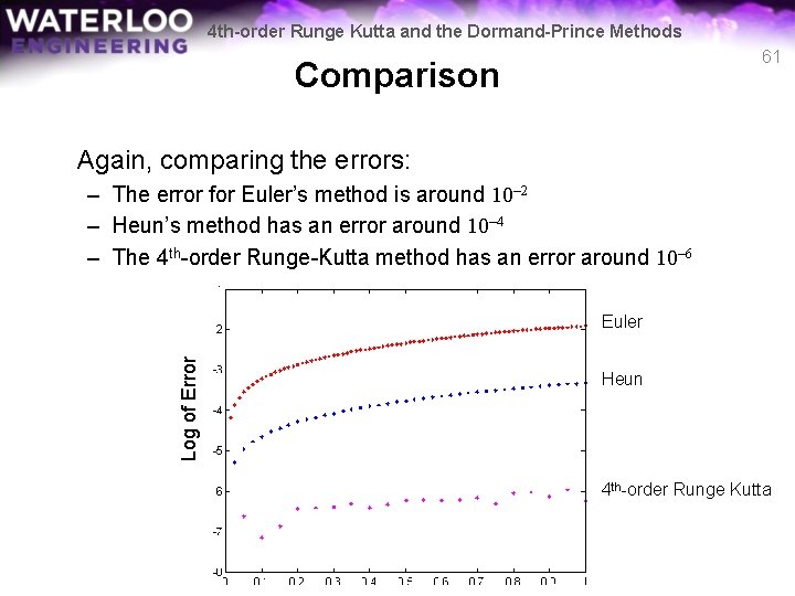
4 th-order Runge Kutta and the Dormand-Prince Methods 61 Comparison Again, comparing the errors: – The error for Euler’s method is around 10– 2 – Heun’s method has an error around 10– 4 – The 4 th-order Runge-Kutta method has an error around 10– 6 Log of Error Euler Heun 4 th-order Runge Kutta

4 th-order Runge Kutta and the Dormand-Prince Methods The Dormand-Prince Method With this general implementation of Runge-Kutta methods, we may now go on to the current algorithm used in Matlab today – The routine ode 45 uses the Dormand-Prince method 62

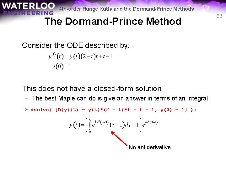
4 th-order Runge Kutta and the Dormand-Prince Methods The Dormand-Prince Method Consider the ODE described by: This does not have a closed-form solution – The best Maple can do is give an answer in terms of an integral: > dsolve( {D(y)(t) = y(t)*(2 - t)*t + t - 1, y(0) = 1} ); No antiderivative 63

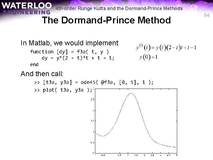
4 th-order Runge Kutta and the Dormand-Prince Methods The Dormand-Prince Method In Matlab, we would implement function [dy] = f 3 a( t, y ) dy = y*(2 - t)*t + t - 1; end And then call: >> [t 3 a, y 3 a] = ode 45( @f 3 a, [0, 5], 1 ); >> plot( t 3 a, y 3 a ); 64

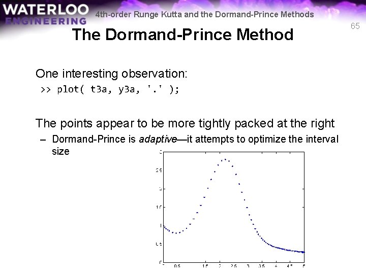
4 th-order Runge Kutta and the Dormand-Prince Methods The Dormand-Prince Method One interesting observation: >> plot( t 3 a, y 3 a, '. ' ); The points appear to be more tightly packed at the right – Dormand-Prince is adaptive—it attempts to optimize the interval size 65

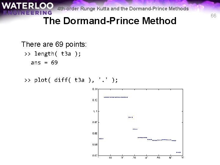
4 th-order Runge Kutta and the Dormand-Prince Methods The Dormand-Prince Method There are 69 points: >> length( t 3 a ); ans = 69 >> plot( diff( t 3 a ), '. ' ); 66

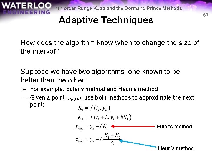
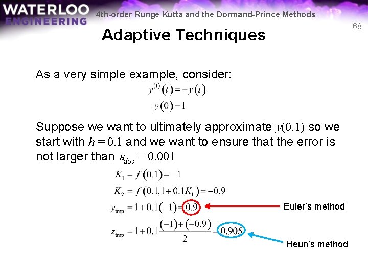
4 th-order Runge Kutta and the Dormand-Prince Methods 67 Adaptive Techniques How does the algorithm know when to change the size of the interval? Suppose we have two algorithms, one known to be better than the other: – For example, Euler’s method and Heun’s method – Given a point (tk, yk), use both methods to approximate the next point: Euler’s method Heun’s method

4 th-order Runge Kutta and the Dormand-Prince Methods 68 Adaptive Techniques As a very simple example, consider: Suppose we want to ultimately approximate y(0. 1) so we start with h = 0. 1 and we want to ensure that the error is not larger than eabs = 0. 001 Euler’s method Heun’s method

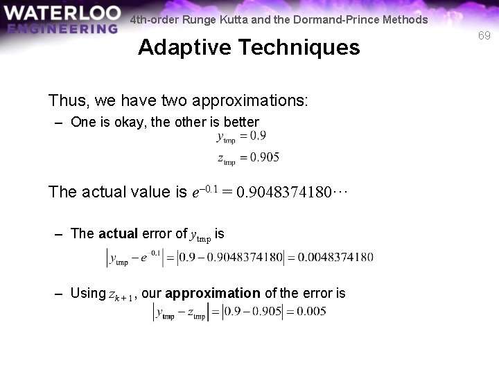
4 th-order Runge Kutta and the Dormand-Prince Methods Adaptive Techniques Thus, we have two approximations: – One is okay, the other is better The actual value is e– 0. 1 = 0. 9048374180··· – The actual error of ytmp is – Using zk + 1, our approximation of the error is 69

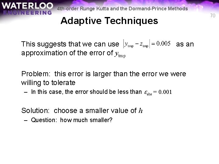
4 th-order Runge Kutta and the Dormand-Prince Methods 70 Adaptive Techniques This suggests that we can use approximation of the error of ytmp as an Problem: this error is larger than the error we were willing to tolerate – In this case, the error should be less than eabs = 0. 001 Solution: choose a smaller value of h – Question: how much smaller?

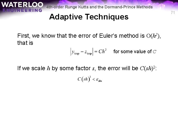
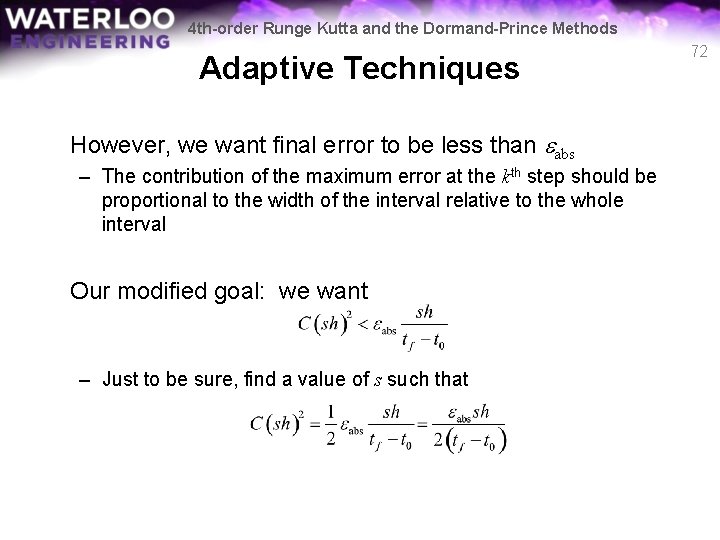
4 th-order Runge Kutta and the Dormand-Prince Methods Adaptive Techniques First, we know that the error of Euler’s method is O(h 2), that is for some value of C If we scale h by some factor s, the error will be C(sh)2: 71

4 th-order Runge Kutta and the Dormand-Prince Methods Adaptive Techniques However, we want final error to be less than eabs – The contribution of the maximum error at the kth step should be proportional to the width of the interval relative to the whole interval Our modified goal: we want – Just to be sure, find a value of s such that 72

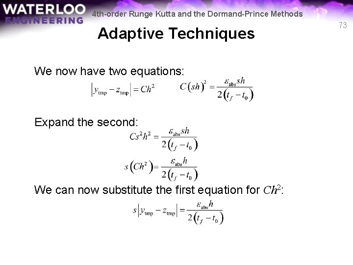
4 th-order Runge Kutta and the Dormand-Prince Methods Adaptive Techniques We now have two equations: Expand the second: We can now substitute the first equation for Ch 2: 73

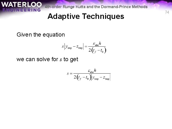
4 th-order Runge Kutta and the Dormand-Prince Methods Adaptive Techniques Given the equation we can solve for s to get 74

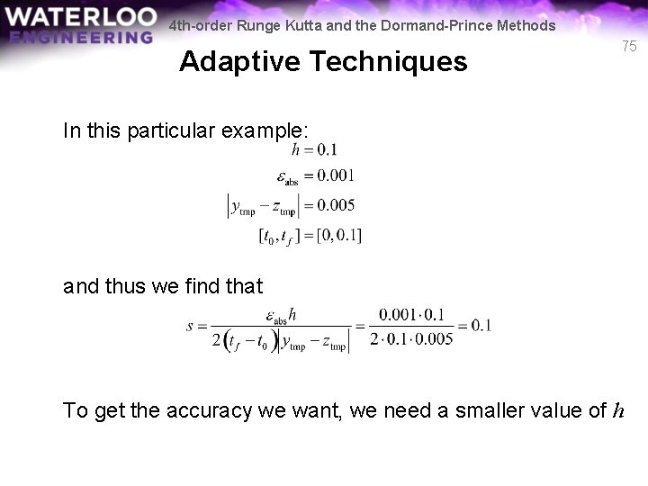
4 th-order Runge Kutta and the Dormand-Prince Methods Adaptive Techniques 75 In this particular example: and thus we find that To get the accuracy we want, we need a smaller value of h

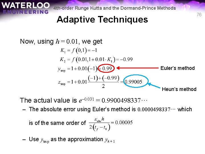
4 th-order Runge Kutta and the Dormand-Prince Methods 76 Adaptive Techniques Now, using h = 0. 01, we get Euler’s method Heun’s method The actual value is e– 0. 031 = 0. 9900498337··· – The absolute error using Euler’s method is 0. 0000498337··· which is of the same order of – Use ytmp as the approximation yk + 1

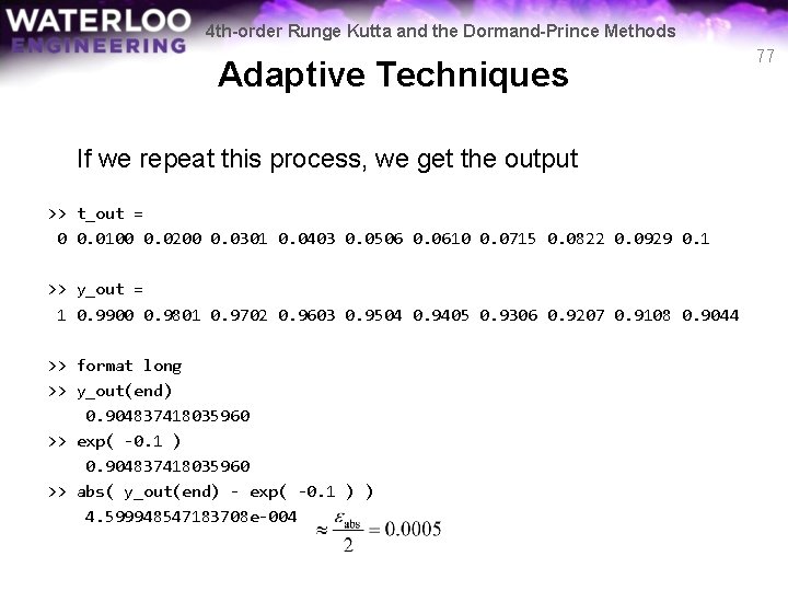
4 th-order Runge Kutta and the Dormand-Prince Methods Adaptive Techniques If we repeat this process, we get the output >> t_out = 0 0. 0100 0. 0200 0. 0301 0. 0403 0. 0506 0. 0610 0. 0715 0. 0822 0. 0929 0. 1 >> y_out = 1 0. 9900 0. 9801 0. 9702 0. 9603 0. 9504 0. 9405 0. 9306 0. 9207 0. 9108 0. 9044 >> format long >> y_out(end) 0. 904837418035960 >> exp( -0. 1 ) 0. 904837418035960 >> abs( y_out(end) - exp( -0. 1 ) ) 4. 599948547183708 e-004 77

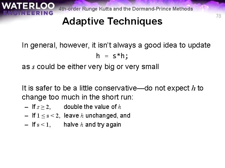
4 th-order Runge Kutta and the Dormand-Prince Methods Adaptive Techniques In general, however, it isn’t always a good idea to update h = s*h; as s could be either very big or very small It is safer to be a little conservative—do not expect h to change too much in the short run: – If s ≥ 2, double the value of h – If 1 ≤ s < 2, leave h unchanged, and – If s < 1, halve h and try again 78

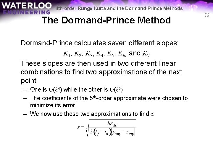
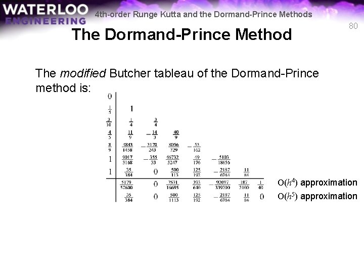
4 th-order Runge Kutta and the Dormand-Prince Methods The Dormand-Prince Method Dormand-Prince calculates seven different slopes: K 1, K 2, K 3, K 4, K 5, K 6, and K 7 These slopes are then used in two different linear combinations to find two approximations of the next point: – One is O(h 4) while the other is O(h 5) – The coefficients of the 5 th-order approximate were chosen to minimize its error – We now use these two approximations to find s: 79

4 th-order Runge Kutta and the Dormand-Prince Methods The Dormand-Prince Method 80 The modified Butcher tableau of the Dormand-Prince method is: O(h 4) approximation O(h 5) approximation

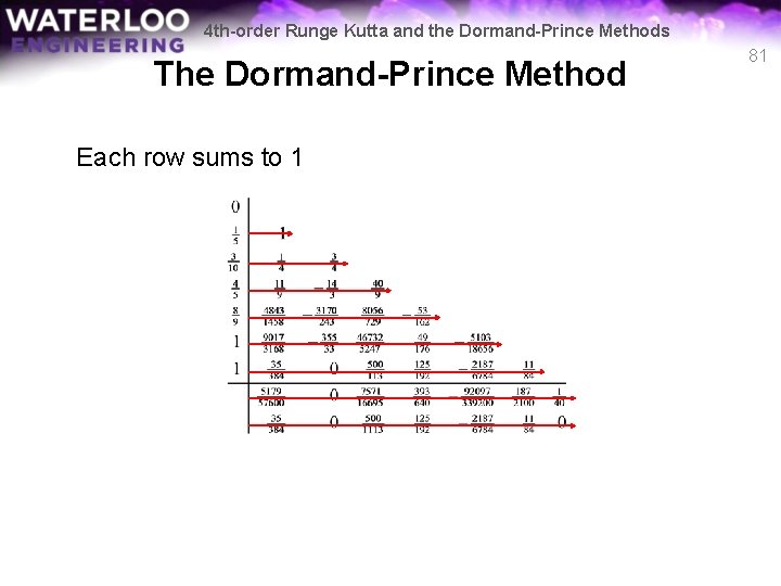
4 th-order Runge Kutta and the Dormand-Prince Methods The Dormand-Prince Method Each row sums to 1 81

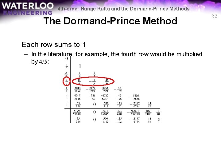
4 th-order Runge Kutta and the Dormand-Prince Methods The Dormand-Prince Method Each row sums to 1 – In the literature, for example, the fourth row would be multiplied by 4/5: 82

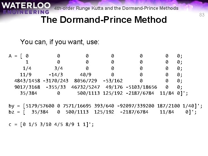
4 th-order Runge Kutta and the Dormand-Prince Methods 83 The Dormand-Prince Method You can, if you want, use: A = [ 0 0 0 1/4 3/4 0 0 11/9 -14/3 40/9 0 0 0 4843/1458 -3170/243 8056/729 -53/162 0 0 9017/3168 -355/33 46732/5247 49/176 -5103/18656 0 35/384 0 500/1113 125/192 -2187/6784 11/84 0; 0; 0; 0]'; by = [5179/57600 0 7571/16695 393/640 -92097/339200 187/2100 1/40]'; bz = [ 35/384 0 500/1113 125/192 -2187/6784 11/84 0]'; c = [0 1/5 3/10 4/5 8/9 1 1]';

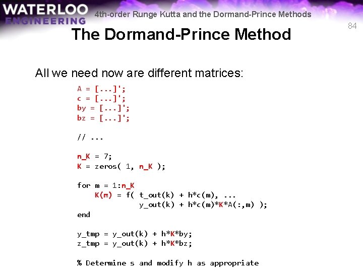
4 th-order Runge Kutta and the Dormand-Prince Methods The Dormand-Prince Method All we need now are different matrices: A = [. . . ]'; c = [. . . ]'; by = [. . . ]'; bz = [. . . ]'; //. . . n_K = 7; K = zeros( 1, n_K ); for m = 1: n_K K(m) = f( t_out(k) + h*c(m), . . . y_out(k) + h*c(m)*K*A(: , m) ); end y_tmp = y_out(k) + h*K*by; z_tmp = y_out(k) + h*K*bz; % Determine s and modify h as appropriate 84

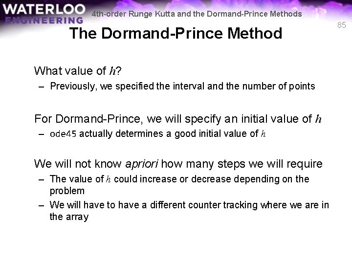
4 th-order Runge Kutta and the Dormand-Prince Methods The Dormand-Prince Method What value of h? – Previously, we specified the interval and the number of points For Dormand-Prince, we will specify an initial value of h – ode 45 actually determines a good initial value of h We will not know apriori how many steps we will require – The value of h could increase or decrease depending on the problem – We will have to have a different counter tracking where we are in the array 85

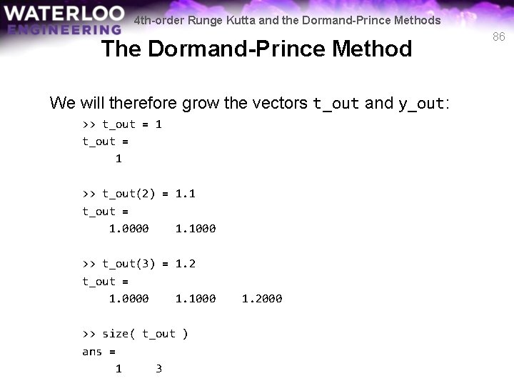
4 th-order Runge Kutta and the Dormand-Prince Methods The Dormand-Prince Method We will therefore grow the vectors t_out and y_out: >> t_out = 1 >> t_out(2) = 1. 1 t_out = 1. 0000 1. 1000 >> t_out(3) = 1. 2 t_out = 1. 0000 1. 1000 >> size( t_out ) ans = 1 3 1. 2000 86

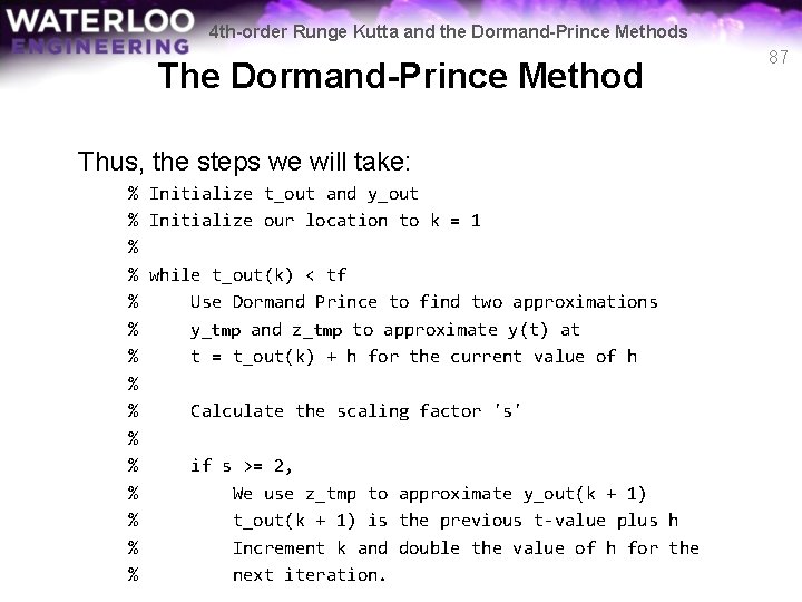
4 th-order Runge Kutta and the Dormand-Prince Methods The Dormand-Prince Method Thus, the steps we will take: % Initialize t_out and y_out % Initialize our location to k = 1 % % while t_out(k) < tf % Use Dormand Prince to find two approximations % y_tmp and z_tmp to approximate y(t) at % t = t_out(k) + h for the current value of h % % Calculate the scaling factor 's' % % if s >= 2, % We use z_tmp to approximate y_out(k + 1) % t_out(k + 1) is the previous t-value plus h % Increment k and double the value of h for the % next iteration. 87

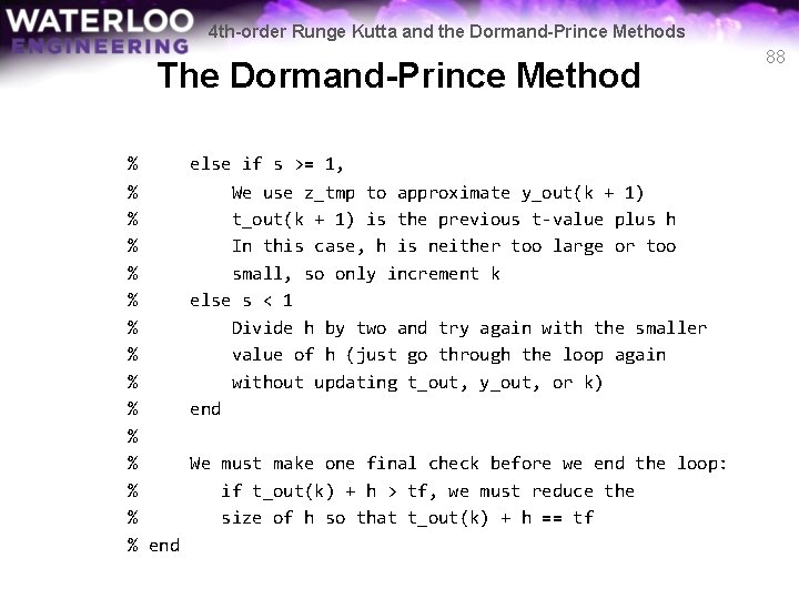
4 th-order Runge Kutta and the Dormand-Prince Methods The Dormand-Prince Method % else if s >= 1, % We use z_tmp to approximate y_out(k + 1) % t_out(k + 1) is the previous t-value plus h % In this case, h is neither too large or too % small, so only increment k % else s < 1 % Divide h by two and try again with the smaller % value of h (just go through the loop again % without updating t_out, y_out, or k) % end % % We must make one final check before we end the loop: % if t_out(k) + h > tf, we must reduce the % size of h so that t_out(k) + h == tf % end 88

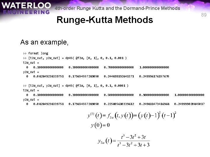
4 th-order Runge Kutta and the Dormand-Prince Methods Runge-Kutta Methods 89 As an example, >> format long >> [t 2 a_out, y 2 a_out] = dp 45( @f 2 a, [0, 1], 0, 0. 1, 0. 001 ) t 2 a_out = 0 0. 10000000 0. 30000000 0. 70000000 y 2 a_out = 0 0. 082849238339751 0. 179654557289050 0. 244899192641371 >> [t 2 a_out, y 2 a_out] = dp 45( @f 2 a, [0, 1], 0, 0. 1, 0. 0001 ) t 2 a_out = 0 0. 10000000 0. 30000000 0. 50000000 y 2 a_out = 0 0. 082849238339751 0. 179654557289050 0. 225805610339612 1. 00000000 0. 249996176157670 0. 90000000 1. 00000000 0. 249811473416968 0. 249999020845017

4 th-order Runge Kutta and the Dormand-Prince Methods Runge-Kutta Methods In the 2 nd example, the values of K, y, z, and s at the four steps are t 1 = 0. 0 h = 0. 1 Approximating t 2 = 0. 1 ytmp = 0. 082849167706690 ztmp = 0. 082849238339751 s = 2. 900617713421327 Note: y 2 a(0. 1) = 0. 082849281565271 Note: double the value of h for the next interval. . . 90

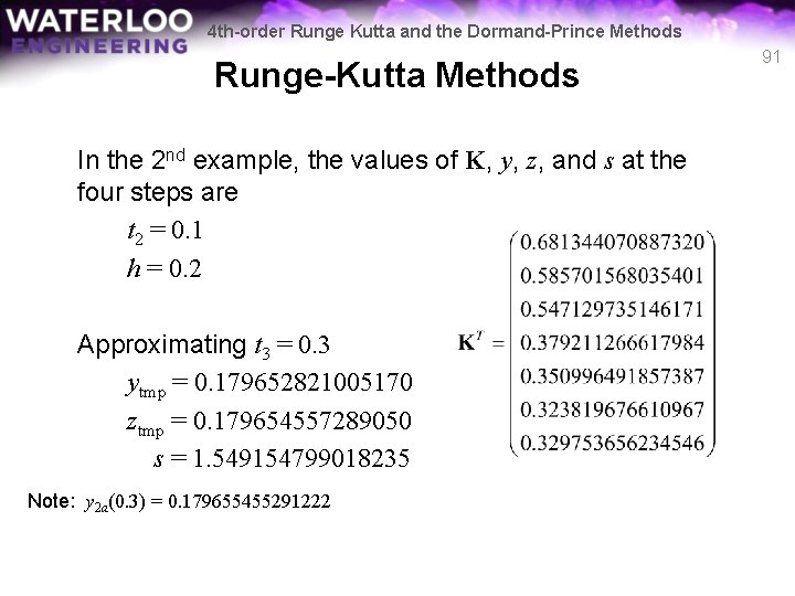
4 th-order Runge Kutta and the Dormand-Prince Methods Runge-Kutta Methods In the 2 nd example, the values of K, y, z, and s at the four steps are t 2 = 0. 1 h = 0. 2 Approximating t 3 = 0. 3 ytmp = 0. 179652821005170 ztmp = 0. 179654557289050 s = 1. 549154799018235 Note: y 2 a(0. 3) = 0. 179655455291222 91

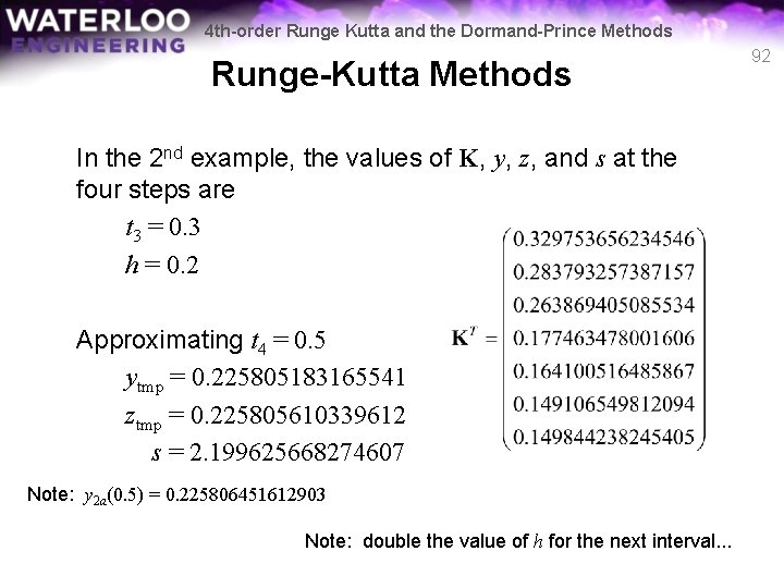
4 th-order Runge Kutta and the Dormand-Prince Methods Runge-Kutta Methods In the 2 nd example, the values of K, y, z, and s at the four steps are t 3 = 0. 3 h = 0. 2 Approximating t 4 = 0. 5 ytmp = 0. 225805183165541 ztmp = 0. 225805610339612 s = 2. 199625668274607 Note: y 2 a(0. 5) = 0. 225806451612903 Note: double the value of h for the next interval. . . 92

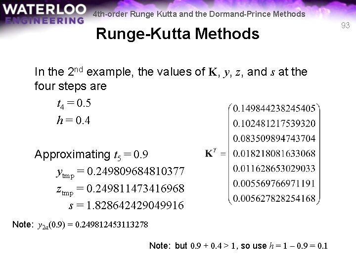
4 th-order Runge Kutta and the Dormand-Prince Methods Runge-Kutta Methods In the 2 nd example, the values of K, y, z, and s at the four steps are t 4 = 0. 5 h = 0. 4 Approximating t 5 = 0. 9 ytmp = 0. 249809684810377 ztmp = 0. 249811473416968 s = 1. 828642429049916 Note: y 2 a(0. 9) = 0. 249812453113278 Note: but 0. 9 + 0. 4 > 1, so use h = 1 – 0. 9 = 0. 1 93

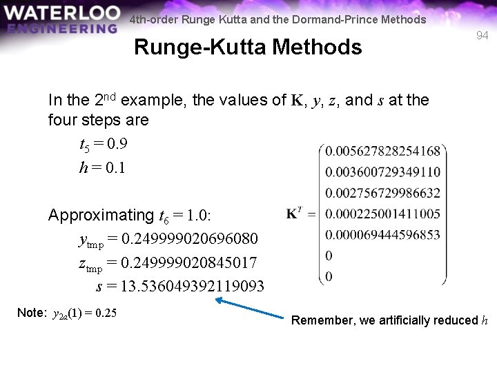
4 th-order Runge Kutta and the Dormand-Prince Methods Runge-Kutta Methods 94 In the 2 nd example, the values of K, y, z, and s at the four steps are t 5 = 0. 9 h = 0. 1 Approximating t 6 = 1. 0: ytmp = 0. 249999020696080 ztmp = 0. 249999020845017 s = 13. 536049392119093 Note: y 2 a(1) = 0. 25 Remember, we artificially reduced h

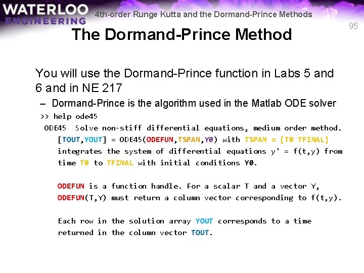
4 th-order Runge Kutta and the Dormand-Prince Methods The Dormand-Prince Method You will use the Dormand-Prince function in Labs 5 and 6 and in NE 217 – Dormand-Prince is the algorithm used in the Matlab ODE solver >> help ode 45 ODE 45 Solve non-stiff differential equations, medium order method. [TOUT, YOUT] = ODE 45(ODEFUN, TSPAN, Y 0) with TSPAN = [T 0 TFINAL] integrates the system of differential equations y' = f(t, y) from time T 0 to TFINAL with initial conditions Y 0. ODEFUN is a function handle. For a scalar T and a vector Y, ODEFUN(T, Y) must return a column vector corresponding to f(t, y). Each row in the solution array YOUT corresponds to a time returned in the column vector TOUT. 95

4 th-order Runge Kutta and the Dormand-Prince Methods Summary We have looked at solving initial-value problems with better techniques: – – Weighted averages and integration techniques 4 th-order Runge Kutta Adaptive methods The Dormand-Prince method 96

4 th-order Runge Kutta and the Dormand-Prince Methods References [1] Glyn James, Modern Engineering Mathematics, 4 th Ed. , Prentice Hall, 2007. [2] Glyn James, Advanced Modern Engineering Mathematics, 4 th Ed. , Prentice Hall, 2011. [3] J. R. Dormand P. J. Prince, "A family of embedded Runge-Kutta formulae, " J. Comp. Appl. Math. , Vol. 6, 1980, pp. 19 -26. 97