4 Simulated Annealing XinShe Yang NatureInspired Optimization Algorithms

4 Simulated Annealing Xin-She Yang, Nature-Inspired Optimization Algorithms, Elsevier, 2014

• Simulated annealing (SA) is a trajectory-based, random search technique for global optimization. • It mimics the annealing process in materials processing when a metal cools and freezes into a crystalline state with the minimum energy and larger crystal sizes so as to reduce the defects in metallic structures.

• The annealing process involves the careful control of temperature and its cooling rate, often called the annealing schedule.

4. 1 Annealing and Boltzmann Distribution • Simulated annealing was proposed by Kirkpatrick et al. in 1983. • The metaphor of SA came from the annealing characteristics in metal processing.

• Unlike the gradient-based methods and other deterministic search methods that have the disadvantage of being trapped into local minima, SA’s main advantage is its ability to avoid being trapped in local minima. • In fact, it has been proved that simulated annealing will converge to its global optimality if enough randomness is used in combination with very slow cooling.

• Metaphorically speaking, this is equivalent to dropping some bouncing balls over a landscape, and as the balls bounce and lose energy, they settle down to some local minima. • If the balls are allowed to bounce enough times and lose energy slowly enough, some of the balls will eventually fall into the globally lowest locations; hence the global minimum can be reached.

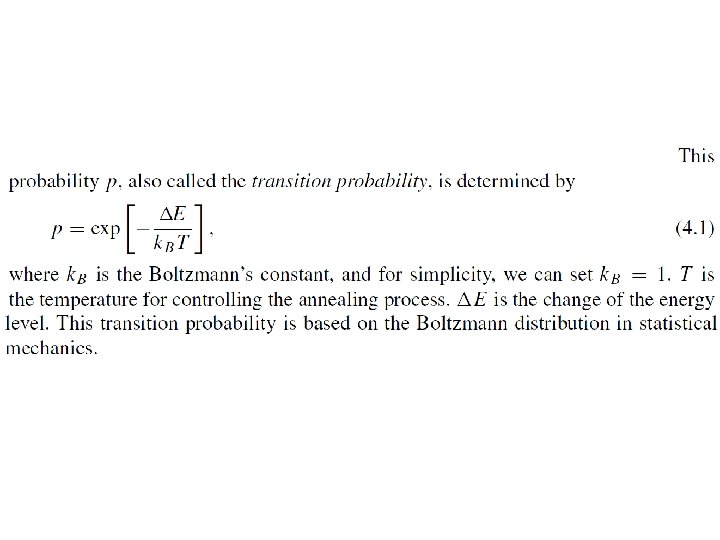
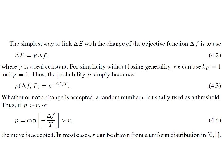
• The basic idea of the SA algorithm is to use random search in terms of a Markov chain, which not only accepts changes that improve the objective function but also keeps some changes that are not ideal. • In a minimization problem, for example, any better moves or changes that decrease the value of the objective function f will be accepted; however, some changes that increase f will also be accepted with a probability p.

4. 2 Parameters • Here the choice of the right initial temperature is crucially important. • For a given change Δf , if T is too high (T → ∞), then p → 1, which means almost all the changes will be accepted. – Random walk • If T is too low (T → 0), then any Δ f > 0 (worse solution) will rarely be accepted as p → 0. – Gradient-based method

• If T is too high, the system is at a high energy state on the topological landscape, and the minima are not easily reached. • If T is too low, the system may be trapped in a local minimum (not necessarily the global minimum), and there is not enough energy for the system to jump out the local minimum to explore other minima, including the global minimum. • So, a proper initial temperature should be calculated.

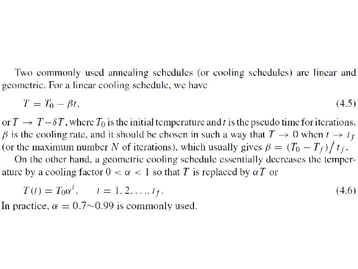
• Another important issue is how to control the annealing or cooling process so that the system cools down gradually from a higher temperature to ultimately freeze to a global minimum state. • There are many ways of controlling the cooling rate or the decrease of the temperature.

• In addition, for a given temperature, multiple evaluations of the objective function are needed. • If there are too few evaluations, there is a danger that the system will not stabilize and subsequently will not converge to its global optimality. • If there are too many evaluations, it is timeconsuming, and the system will usually converge too slowly.

• There are two major ways to set the number of iterations: fixed or varied. • The first uses a fixed number of iterations at each temperature. • The second intends to increase the number of iterations at lower temperatures so that the local minima can be fully explored.

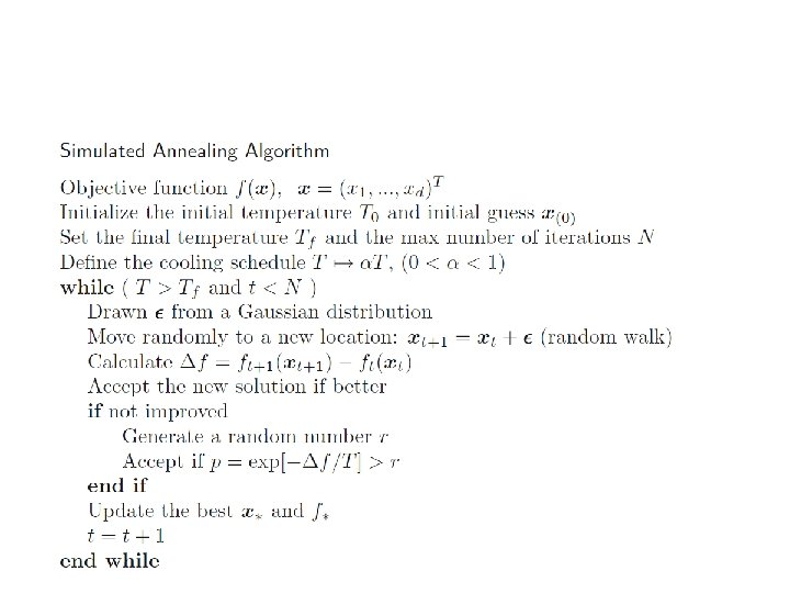
4. 3 SA Algorithm

• Pseudo code appears not entirely correct. There should be multiple evaluations for a particular temperature.