4 Random Variables A random variable is a

4. Random Variables A random variable is a way of recording a quantitative variable of a random experiment.

4. Random Variables A random variable is a way of recording a quantitative variable of a random experiment. In particular Chapter 4 talks about discrete random variables.

4. Random Variables A random variable is a way of recording a quantitative variable of a random experiment. In particular Chapter 4 talks about discrete random variables. If a random variable has a particular distribution (such as a binomial distribution) then our work becomes easier. We use formulas and tables.

5. Continuous Random Variables A random variable is a way of recording a quantitative variable of a random experiment. In particular Chapter 4 talks about discrete random variables. If a random variable has a particular distribution (such as a binomial distribution) then our work becomes easier. We use formulas and tables.

5. Continuous Random Variables A random variable where X can take on a range of values, not just particular ones. Examples: Heights Distance a golfer hits the ball with their driver Time to run 100 meters Electricity usage of a home.

Continuous probability distribution functions For a discrete random variable, probabilities are given as a table of values, and the distribution can be graphed as a bar graph. For a continuous random variable, probabilities are specified by a continuous function. The graph of the probability distribution function is a curve.

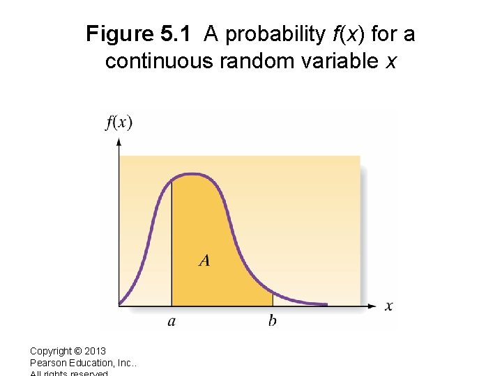
Figure 5. 1 A probability f(x) for a continuous random variable x Copyright ©

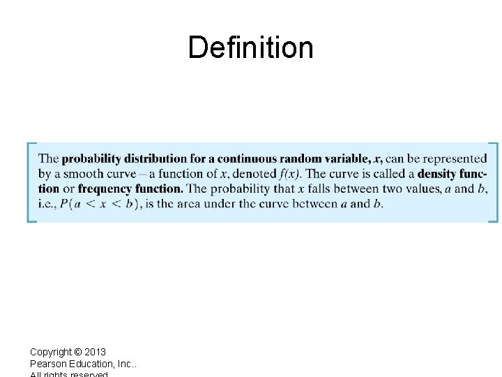
Definition Copyright © 2013 Pearson Education, Inc. .

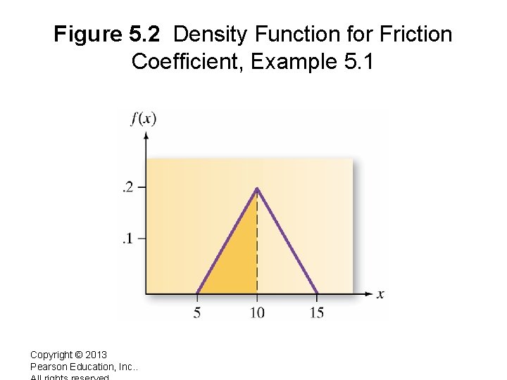
Figure 5. 2 Density Function for Friction Coefficient, Example 5. 1 Copyright © 2013

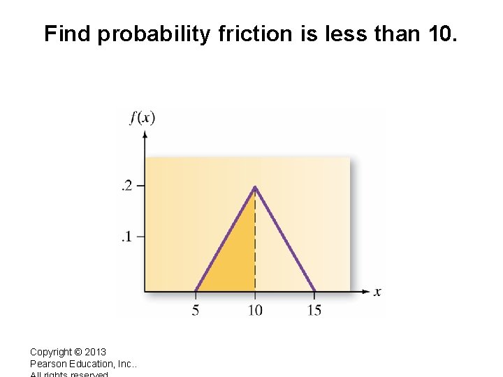
Find probability friction is less than 10. Copyright © 2013 Pearson Education, Inc. .

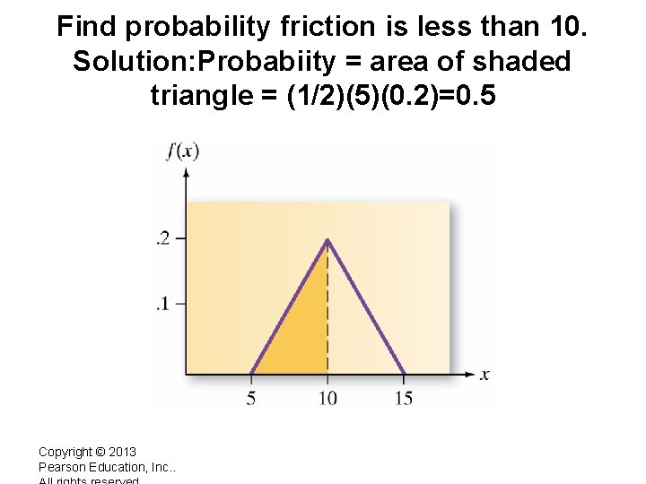
Find probability friction is less than 10. Solution: Probabiity = area of shaded triangle

Uniform Distribution A Uniform Distribution has equally likely values over the range of possible outcomes.

Uniform Distribution A Uniform Distribution has equally likely values over the range of possible outcomes. A graph of the uniform probability distribution is a rectangle with area equal to 1.

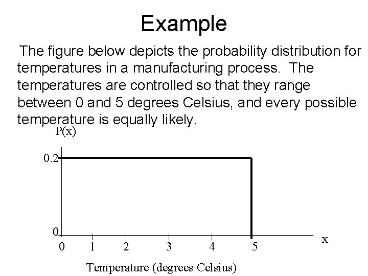
Example The figure below depicts the probability distribution for temperatures in a manufacturing process. The temperatures are controlled so that they range between 0 and 5 degrees Celsius, and every possible temperature is equally likely. P(x) 0. 2 0 0 1 2 3 4 Temperature (degrees Celsius) 5 x

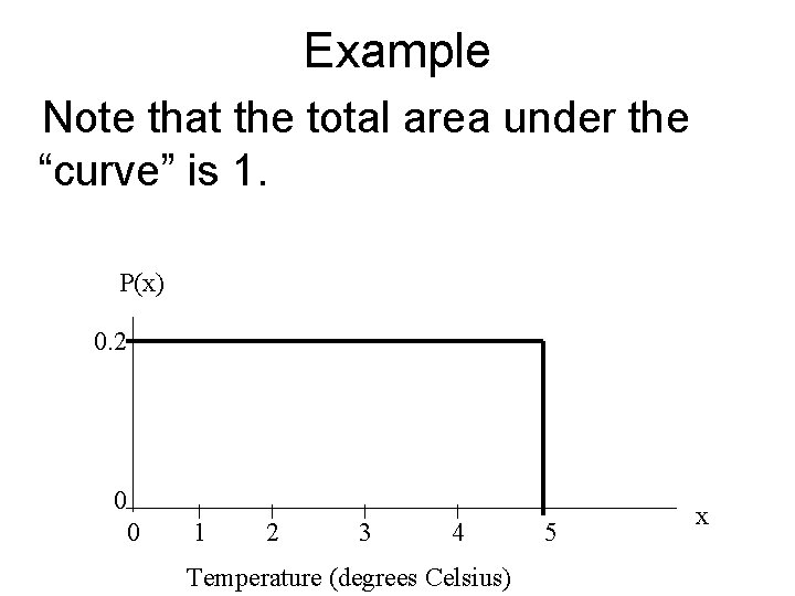
Example Note that the total area under the “curve” is 1. P(x) 0. 2 0 0 1 2 3 4 Temperature (degrees Celsius) 5 x

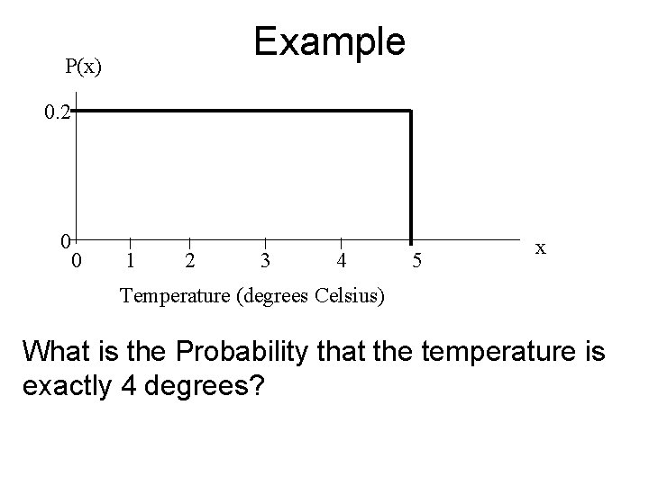
Example P(x) 0. 2 0 0 1 2 3 4 5 x Temperature (degrees Celsius) What is the Probability that the temperature is exactly 4 degrees?

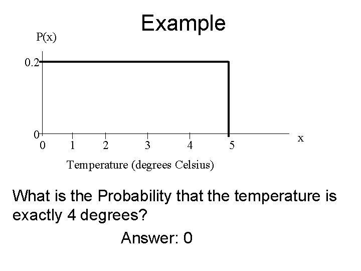
Example P(x) 0. 2 0 0 1 2 3 4 5 x Temperature (degrees Celsius) What is the Probability that the temperature is exactly 4 degrees? Answer: 0

Explanation Since we have a continuous random variable there an infinite number of possible outcomes between 0 and 5, the probability of one number out of an infinite set of numbers is 0.

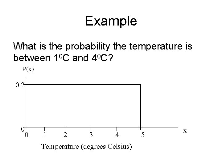
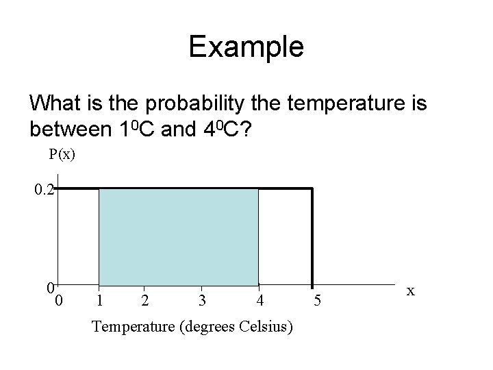
Example What is the probability the temperature is between 10 C and 40 C? P(x) 0. 2 0 0 1 2 3 4 Temperature (degrees Celsius) 5 x

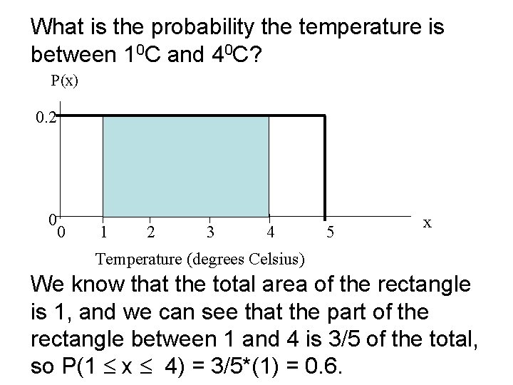
What is the probability the temperature is between 10 C and 40 C? P(x) 0. 2 0 0 1 2 3 4 5 x Temperature (degrees Celsius) We know that the total area of the rectangle is 1, and we can see that the part of the rectangle between 1 and 4 is 3/5 of the total, so P(1 x 4) = 3/5*(1) = 0. 6.

Review: Probabilities and Area For a density curve depicting the probability distribution of a continuous random variable, – the total area under the curve is 1, – there is a direct correspondence between area and probability. – Only the probability of an event occurring in some interval can be evaluated. – The probability that a continuous random variable takes on any particular value is zero.

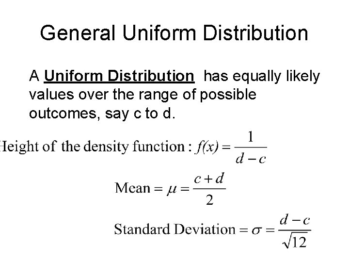
General Uniform Distribution A Uniform Distribution has equally likely values over the range of possible outcomes, say c to d.

Normal Distributions This is the most common observed distribution of continuous random variables. A normal distribution corresponds to bellshaped curves.

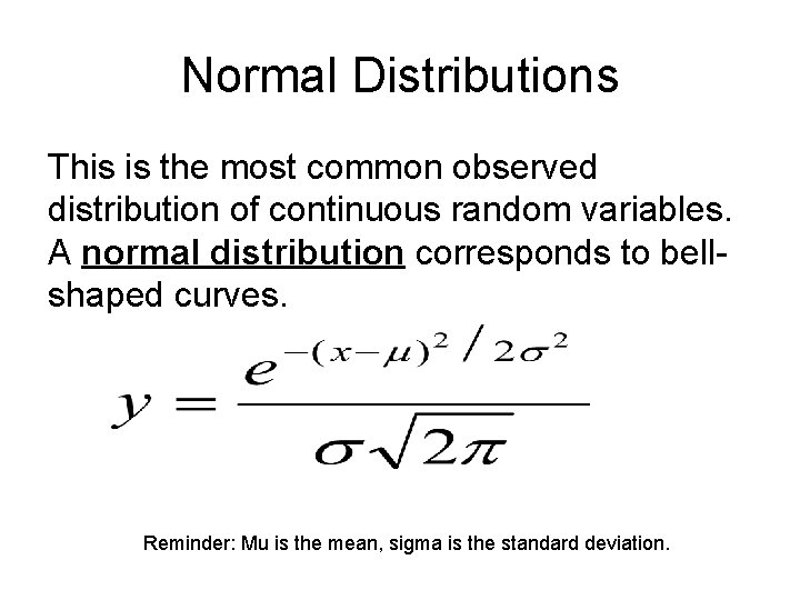
Normal Distributions This is the most common observed distribution of continuous random variables. A normal distribution corresponds to bellshaped curves. Reminder: Mu is the mean, sigma is the standard deviation.

Examples The following are examples of normally distributed everyday data. – Grades on a test. – How many chips are in a small bag of potatoe chips. – The measurements of distance between two points. – The heights of students in this class.

Normal Distributions

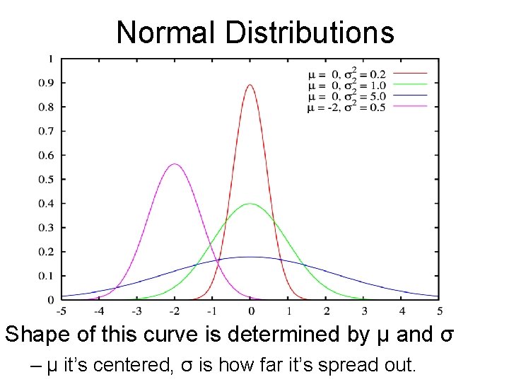
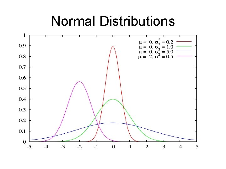
Normal Distributions Shape of this curve is determined by µ and σ – µ it’s centered, σ is how far it’s spread out.

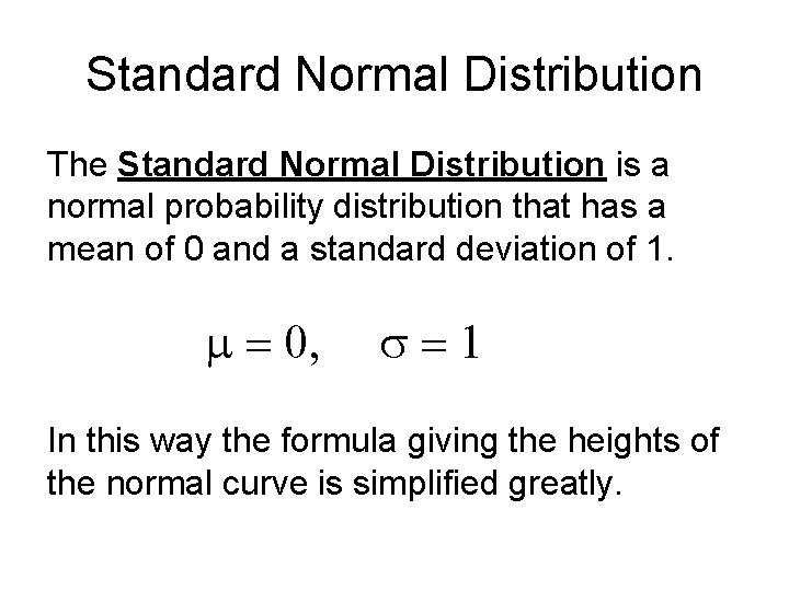
Standard Normal Distribution The Standard Normal Distribution is a normal probability distribution that has a mean of 0 and a standard deviation of 1. m = 0, s=1 In this way the formula giving the heights of the normal curve is simplified greatly.

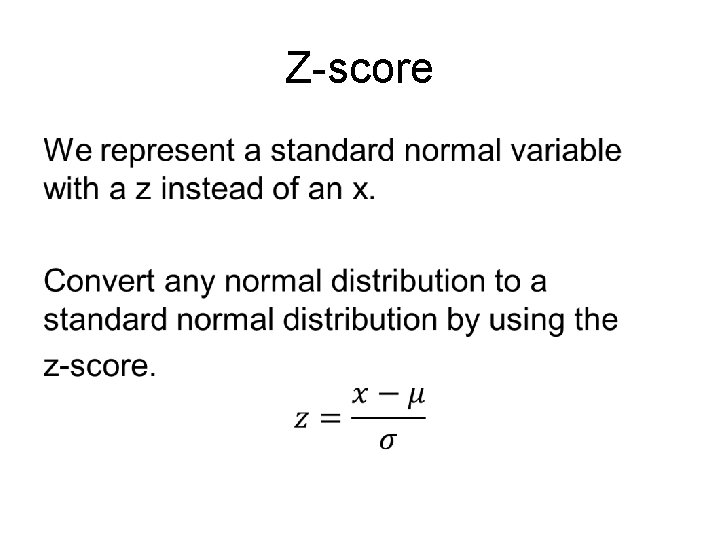
Z-score •

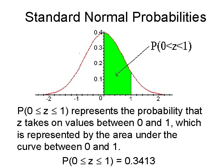
Standard Normal Probabilities P(0 z 1) represents the probability that z takes on values between 0 and 1, which is represented by the area under the curve between 0 and 1. P(0 z 1) = 0. 3413

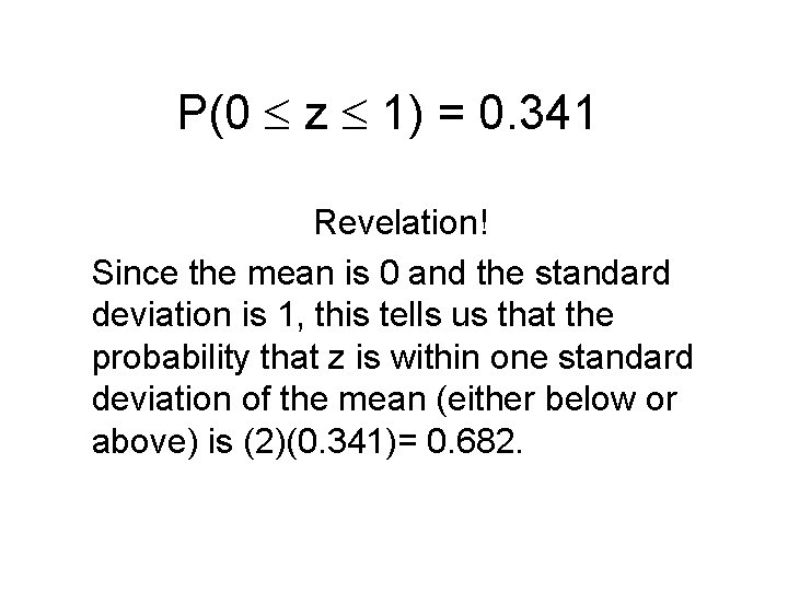
P(0 z 1) = 0. 341 Revelation! Since the mean is 0 and the standard deviation is 1, this tells us that the probability that z is within one standard deviation of the mean (either below or above) is (2)(0. 341)= 0. 682.

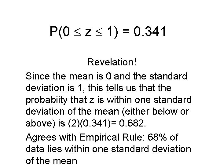
P(0 z 1) = 0. 341 Revelation! Since the mean is 0 and the standard deviation is 1, this tells us that the probabiity that z is within one standard deviation of the mean (either below or above) is (2)(0. 341)= 0. 682. Agrees with Empirical Rule: 68% of data lies within one standard deviation of the mean

Finding Probabilities when given z-scores. For a given z-score, the probability can be found in a table in the back of the text (Table IV), also see inside front cover. Note: The table only gives the areas under the curve to the right between 0 and z. To find other intervals requires some tricks.

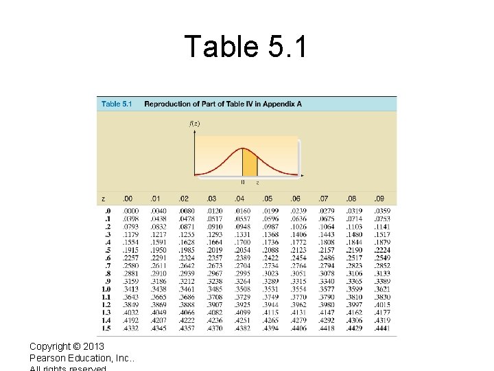
Table 5. 1 Copyright © 2013 Pearson Education, Inc. .

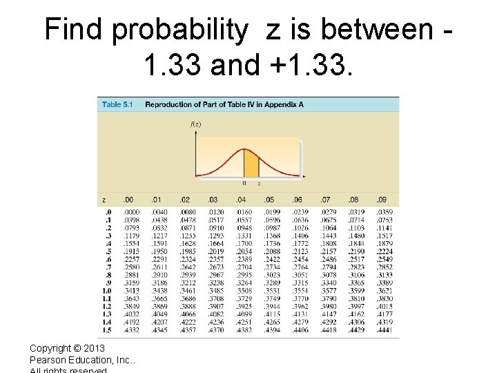
Find probability z is between 1. 33 and +1. 33. Copyright © 2013 Pearson

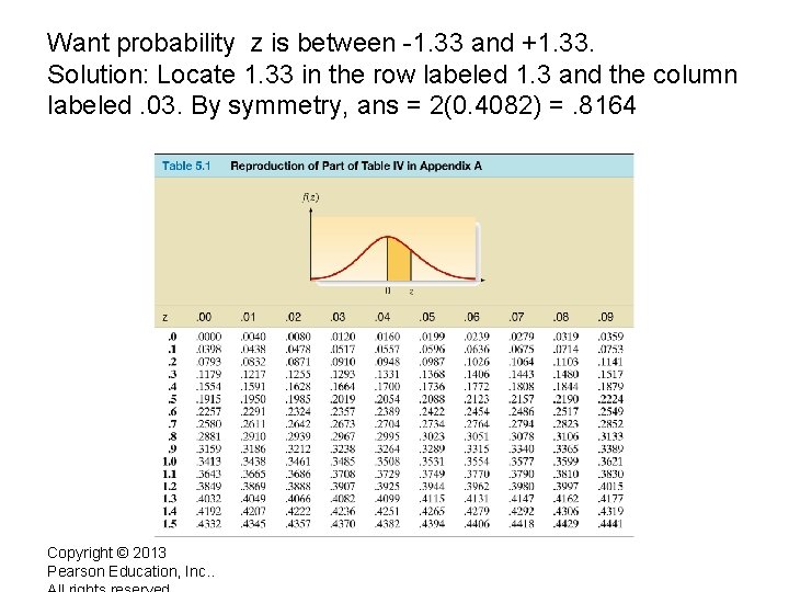
Want probability z is between -1. 33 and +1. 33. Solution: Locate 1. 33 in the row labeled 1. 3 and the column labeled. 03. By symmetry, ans = 2(0. 4082) =. 8164 Copyright © 2013 Pearson Education, Inc. .

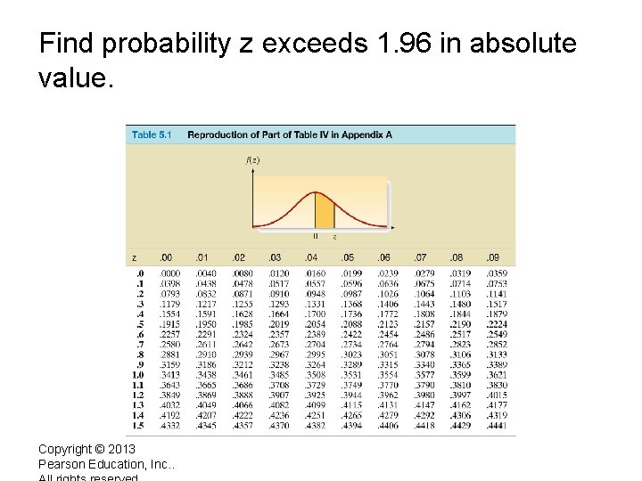
Find probability z exceeds 1. 96 in absolute value. Copyright © 2013 Pearson Education,

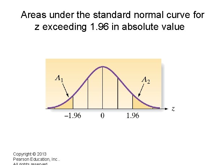
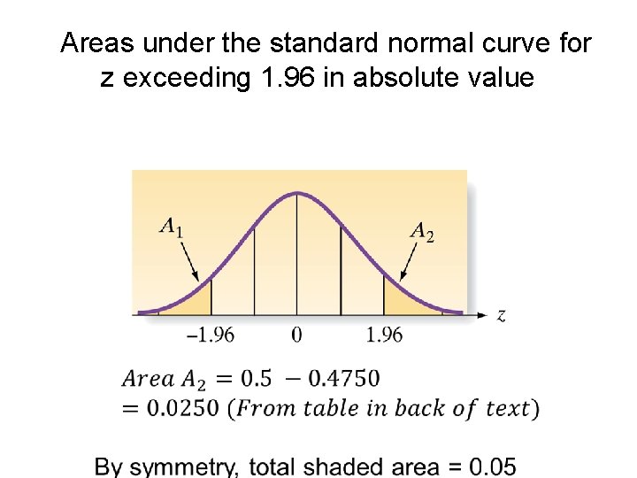
Areas under the standard normal curve for z exceeding 1. 96 in absolute value

Revelation! It follows that the area of the unshaded region is 0. 95. Agrees with Empirical Rule which states that, for data sets having a mound shaped distribution, 95% of the values lie within approximately 2 standard deviations of the mean

Keys to success Learn the standard normal table and how to use it. We will be using these tables through out the course.