4 Integrals Copyright Cengage Learning All rights reserved

4 Integrals Copyright © Cengage Learning. All rights reserved.

4. 1 Areas and Distances Copyright © Cengage Learning. All rights reserved.

The Area Problem 3

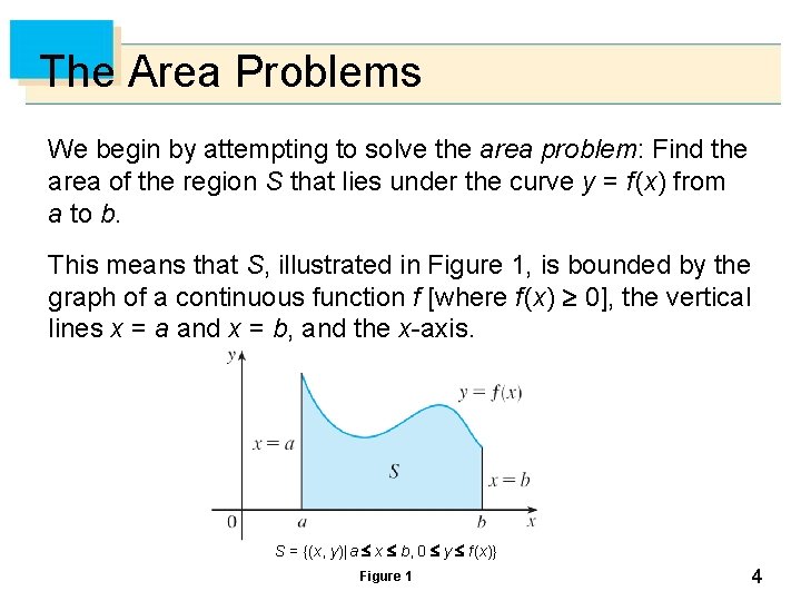
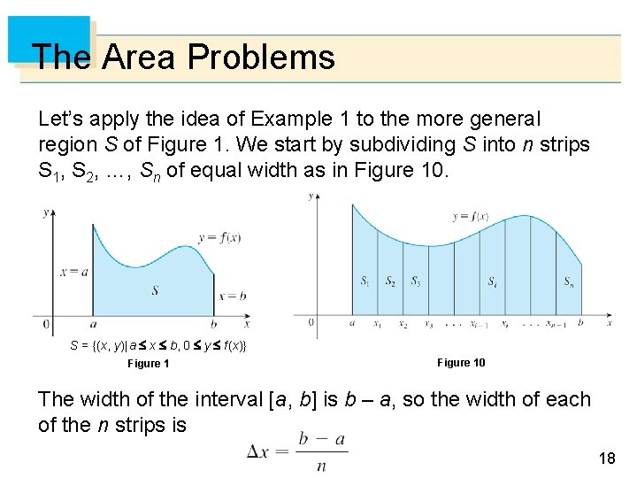
The Area Problems We begin by attempting to solve the area problem: Find the area of the region S that lies under the curve y = f (x) from a to b. This means that S, illustrated in Figure 1, is bounded by the graph of a continuous function f [where f (x) 0], the vertical lines x = a and x = b, and the x-axis. S = {(x, y) | a x b, 0 y f (x)} Figure 1 4

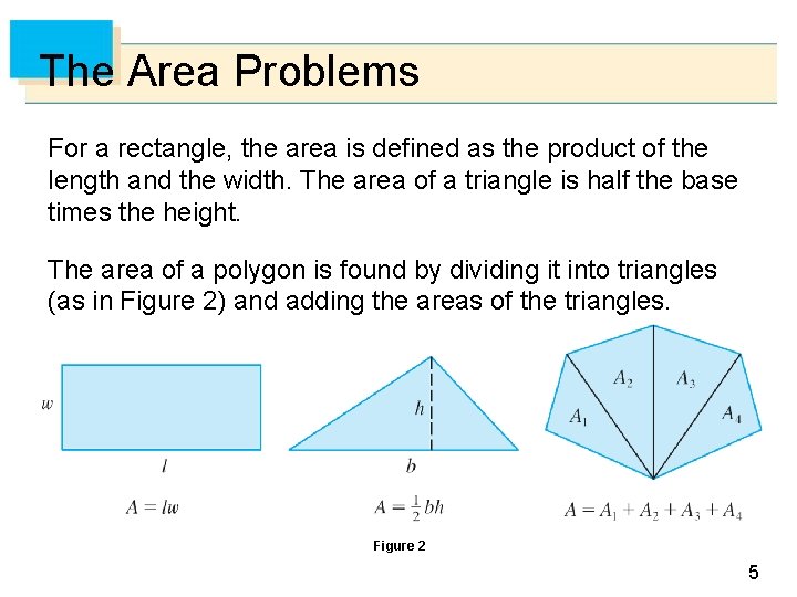
The Area Problems For a rectangle, the area is defined as the product of the length and the width. The area of a triangle is half the base times the height. The area of a polygon is found by dividing it into triangles (as in Figure 2) and adding the areas of the triangles. Figure 2 5

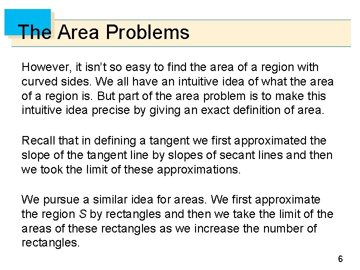
The Area Problems However, it isn’t so easy to find the area of a region with curved sides. We all have an intuitive idea of what the area of a region is. But part of the area problem is to make this intuitive idea precise by giving an exact definition of area. Recall that in defining a tangent we first approximated the slope of the tangent line by slopes of secant lines and then we took the limit of these approximations. We pursue a similar idea for areas. We first approximate the region S by rectangles and then we take the limit of the areas of these rectangles as we increase the number of rectangles. 6

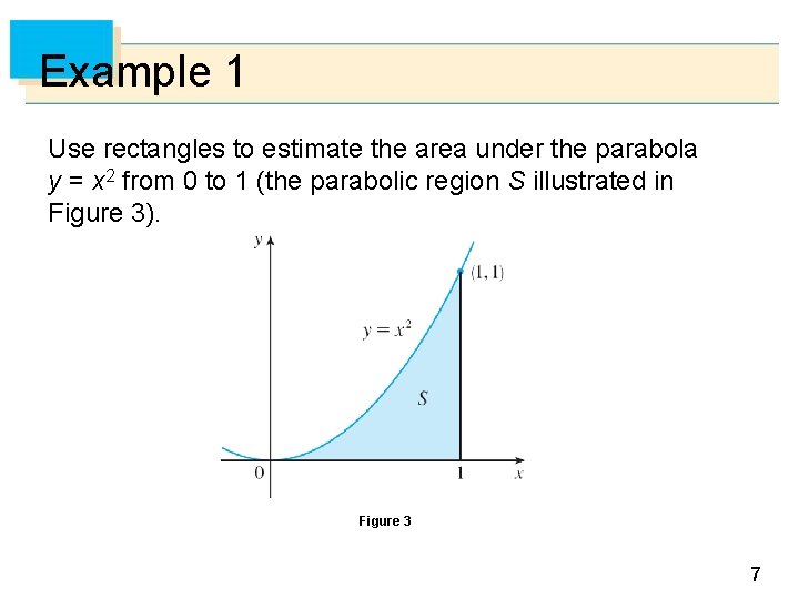
Example 1 Use rectangles to estimate the area under the parabola y = x 2 from 0 to 1 (the parabolic region S illustrated in Figure 3). Figure 3 7

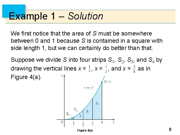
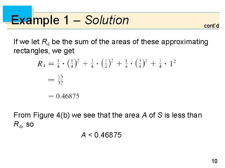
Example 1 – Solution We first notice that the area of S must be somewhere between 0 and 1 because S is contained in a square with side length 1, but we can certainly do better than that. Suppose we divide S into four strips S 1, S 2, S 3, and S 4 by drawing the vertical lines x = , and x = as in Figure 4(a) 8

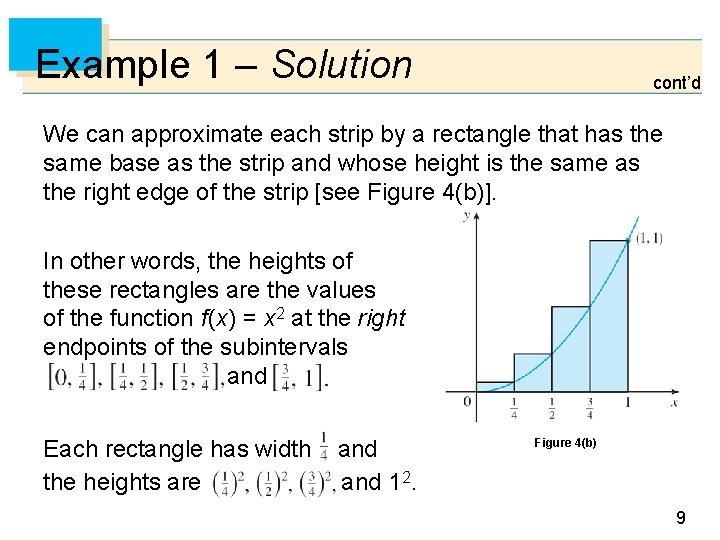
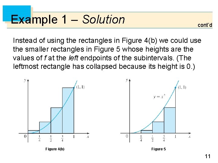
Example 1 – Solution cont’d We can approximate each strip by a rectangle that has the same base as the strip and whose height is the same as the right edge of the strip [see Figure 4(b)]. In other words, the heights of these rectangles are the values of the function f (x) = x 2 at the right endpoints of the subintervals and Each rectangle has width the heights are and 12. Figure 4(b) 9

Example 1 – Solution cont’d If we let R 4 be the sum of the areas of these approximating rectangles, we get From Figure 4(b) we see that the area A of S is less than R 4, so A < 0. 46875 10

Example 1 – Solution cont’d Instead of using the rectangles in Figure 4(b) we could use the smaller rectangles in Figure 5 whose heights are the values of f at the left endpoints of the subintervals. (The leftmost rectangle has collapsed because its height is 0. ) Figure 4(b) Figure 5 11

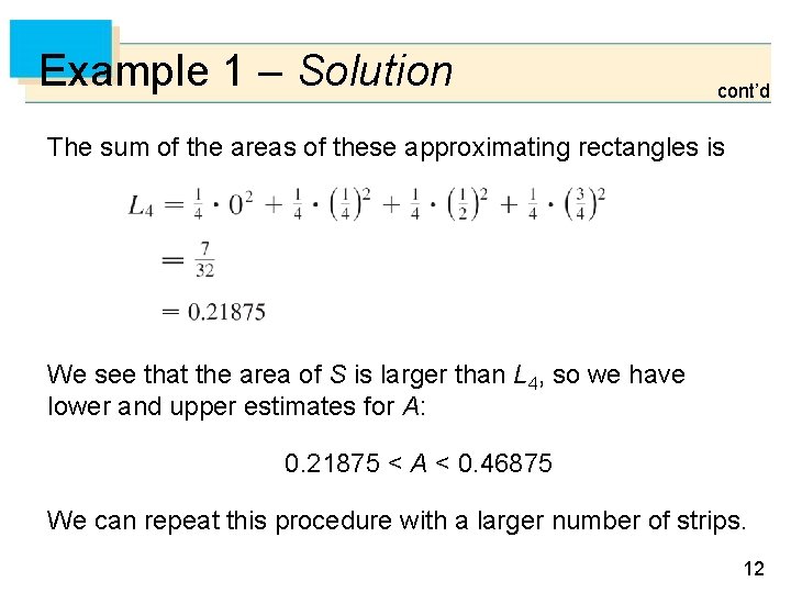
Example 1 – Solution cont’d The sum of the areas of these approximating rectangles is We see that the area of S is larger than L 4, so we have lower and upper estimates for A: 0. 21875 < A < 0. 46875 We can repeat this procedure with a larger number of strips. 12

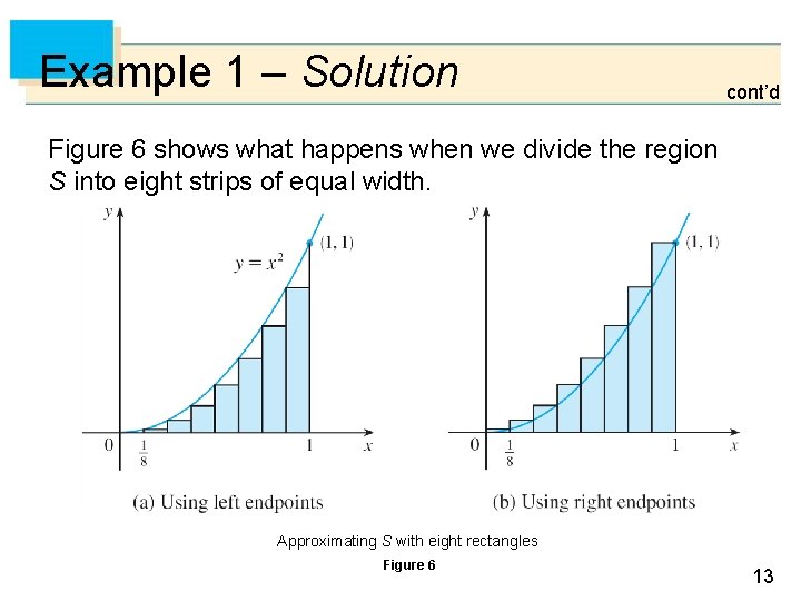
Example 1 – Solution cont’d Figure 6 shows what happens when we divide the region S into eight strips of equal width. Approximating S with eight rectangles Figure 6 13

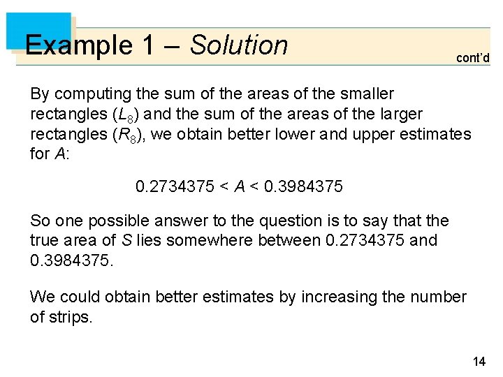
Example 1 – Solution cont’d By computing the sum of the areas of the smaller rectangles (L 8) and the sum of the areas of the larger rectangles (R 8), we obtain better lower and upper estimates for A: 0. 2734375 < A < 0. 3984375 So one possible answer to the question is to say that the true area of S lies somewhere between 0. 2734375 and 0. 3984375. We could obtain better estimates by increasing the number of strips. 14

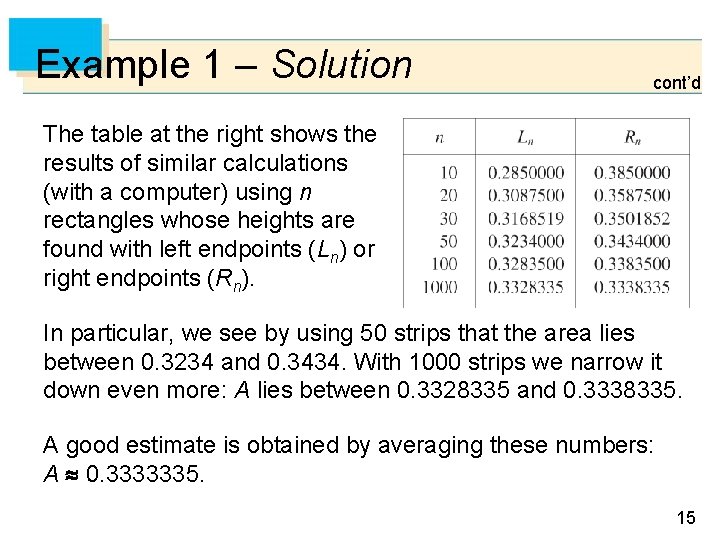
Example 1 – Solution cont’d The table at the right shows the results of similar calculations (with a computer) using n rectangles whose heights are found with left endpoints (Ln) or right endpoints (Rn). In particular, we see by using 50 strips that the area lies between 0. 3234 and 0. 3434. With 1000 strips we narrow it down even more: A lies between 0. 3328335 and 0. 3338335. A good estimate is obtained by averaging these numbers: A 0. 3333335. 15

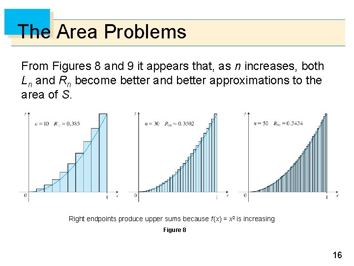
The Area Problems From Figures 8 and 9 it appears that, as n increases, both Ln and Rn become better and better approximations to the area of S. Right endpoints produce upper sums because f (x) = x 2 is increasing Figure 8 16

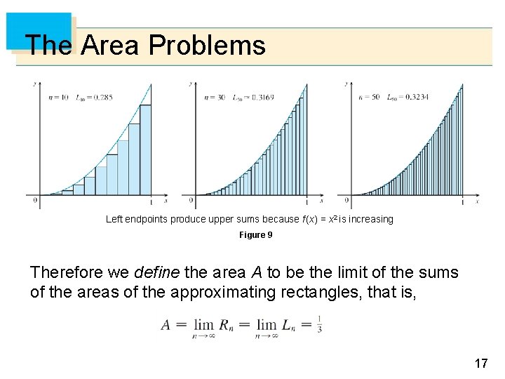
The Area Problems Left endpoints produce upper sums because f (x) = x 2 is increasing Figure 9 Therefore we define the area A to be the limit of the sums of the areas of the approximating rectangles, that is, 17

The Area Problems Let’s apply the idea of Example 1 to the more general region S of Figure 1. We start by subdividing S into n strips S 1, S 2, …, Sn of equal width as in Figure 10. S = {(x, y) | a x b, 0 y f (x)} Figure 10 The width of the interval [a, b] is b – a, so the width of each of the n strips is 18

The Area Problems These strips divide the interval [a, b] into n subintervals [x 0, x 1], [x 1, x 2], [x 2, x 3], . . . , [xn – 1, xn] where x 0 = a and xn = b. The right endpoints of the subintervals are x 1 = a + x, x 2 = a + 2 x, x 3 = a + 3 x, 19

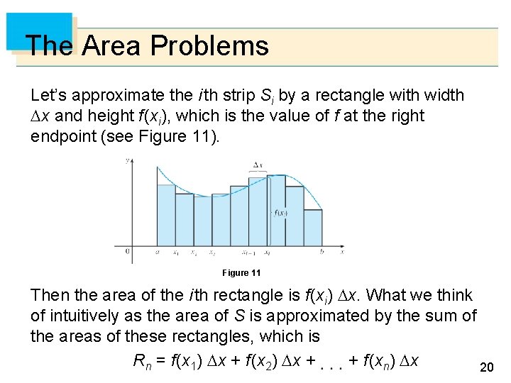
The Area Problems Let’s approximate the i th strip Si by a rectangle with width x and height f (xi), which is the value of f at the right endpoint (see Figure 11). Figure 11 Then the area of the i th rectangle is f (xi) x. What we think of intuitively as the area of S is approximated by the sum of the areas of these rectangles, which is Rn = f (x 1) x + f (x 2) x + + f (xn) x 20

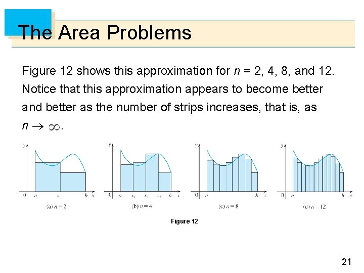
The Area Problems Figure 12 shows this approximation for n = 2, 4, 8, and 12. Notice that this approximation appears to become better and better as the number of strips increases, that is, as n . Figure 12 21

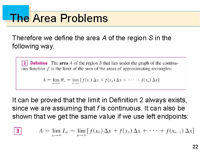
The Area Problems Therefore we define the area A of the region S in the following way. It can be proved that the limit in Definition 2 always exists, since we are assuming that f is continuous. It can also be shown that we get the same value if we use left endpoints: 22

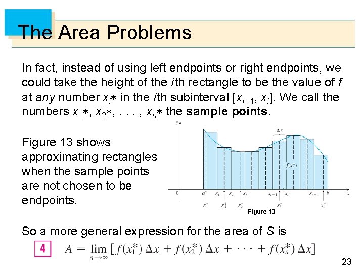
The Area Problems In fact, instead of using left endpoints or right endpoints, we could take the height of the i th rectangle to be the value of f at any number xi in the i th subinterval [xi – 1, xi ]. We call the numbers x 1 , x 2 , . . . , xn the sample points. Figure 13 shows approximating rectangles when the sample points are not chosen to be endpoints. Figure 13 So a more general expression for the area of S is 23

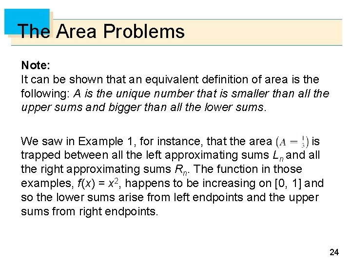
The Area Problems Note: It can be shown that an equivalent definition of area is the following: A is the unique number that is smaller than all the upper sums and bigger than all the lower sums. We saw in Example 1, for instance, that the area is trapped between all the left approximating sums Ln and all the right approximating sums Rn. The function in those examples, f (x) = x 2, happens to be increasing on [0, 1] and so the lower sums arise from left endpoints and the upper sums from right endpoints. 24

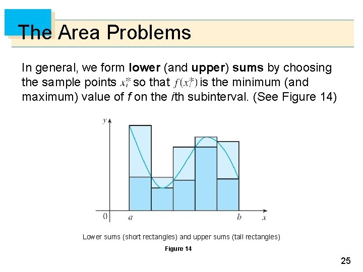
The Area Problems In general, we form lower (and upper) sums by choosing the sample points so that is the minimum (and maximum) value of f on the i th subinterval. (See Figure 14) Lower sums (short rectangles) and upper sums (tall rectangles) Figure 14 25

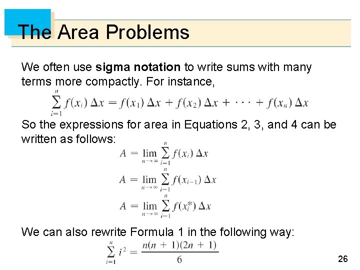
The Area Problems We often use sigma notation to write sums with many terms more compactly. For instance, So the expressions for area in Equations 2, 3, and 4 can be written as follows: We can also rewrite Formula 1 in the following way: 26

The Distance Problem 27

The Distance Problems Now let’s consider the distance problem: Find the distance traveled by an object during a certain time period if the velocity of the object is known at all times. If the velocity remains constant, then the distance problem is easy to solve by means of the formula distance = velocity time But if the velocity varies, it’s not so easy to find the distance traveled. 28

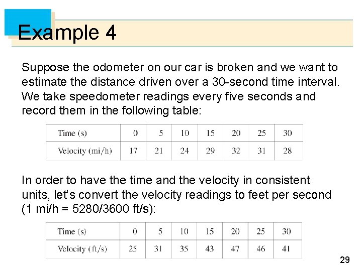
Example 4 Suppose the odometer on our car is broken and we want to estimate the distance driven over a 30 -second time interval. We take speedometer readings every five seconds and record them in the following table: In order to have the time and the velocity in consistent units, let’s convert the velocity readings to feet per second (1 mi/h = 5280/3600 ft/s): 29

Example 4 cont’d During the first five seconds the velocity doesn’t change very much, so we can estimate the distance traveled during that time by assuming that the velocity is constant. If we take the velocity during that time interval to be the initial velocity (25 ft/s), then we obtain the approximate distance traveled during the first five seconds: 25 ft/s 5 s = 125 ft 30

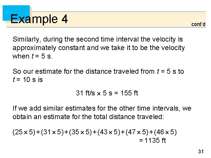
Example 4 cont’d Similarly, during the second time interval the velocity is approximately constant and we take it to be the velocity when t = 5 s. So our estimate for the distance traveled from t = 5 s to t = 10 s is 31 ft/s 5 s = 155 ft If we add similar estimates for the other time intervals, we obtain an estimate for the total distance traveled: (25 5) + (31 5) + (35 5) + (43 5) + (47 5) + (46 5) = 1135 ft 31

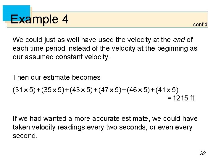
Example 4 cont’d We could just as well have used the velocity at the end of each time period instead of the velocity at the beginning as our assumed constant velocity. Then our estimate becomes (31 5) + (35 5) + (43 5) + (47 5) + (46 5) + (41 5) = 1215 ft If we had wanted a more accurate estimate, we could have taken velocity readings every two seconds, or even every second. 32

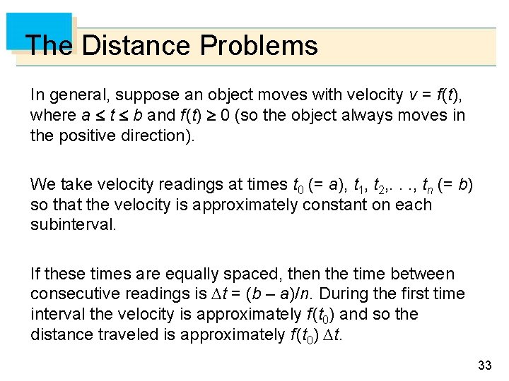
The Distance Problems In general, suppose an object moves with velocity v = f (t), where a t b and f (t) 0 (so the object always moves in the positive direction). We take velocity readings at times t 0 (= a), t 1, t 2, . . . , tn (= b) so that the velocity is approximately constant on each subinterval. If these times are equally spaced, then the time between consecutive readings is t = (b – a)/n. During the first time interval the velocity is approximately f (t 0) and so the distance traveled is approximately f (t 0) t. 33

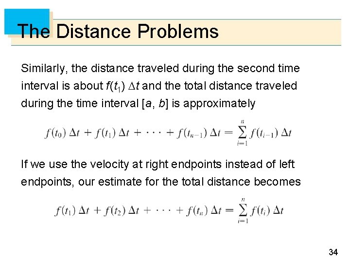
The Distance Problems Similarly, the distance traveled during the second time interval is about f (t 1) t and the total distance traveled during the time interval [a, b] is approximately If we use the velocity at right endpoints instead of left endpoints, our estimate for the total distance becomes 34

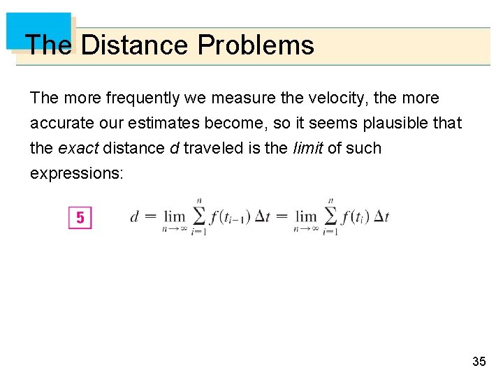
The Distance Problems The more frequently we measure the velocity, the more accurate our estimates become, so it seems plausible that the exact distance d traveled is the limit of such expressions: 35