4 Graphs of the Circular Functions Copyright 2013

4 Graphs of the Circular Functions Copyright © 2013, 2009, 2005 Pearson Education, Inc. 1

4 Graphs of the Circular Functions 4. 1 Graphs of the Sine and Cosine Functions 4. 2 Translations of the Graphs of the Sine and Cosine Functions 4. 3 Graphs of the Tangent and Cotangent Functions 4. 4 Graphs of the Secant and Cosecant Functions Copyright © 2013, 2009, 2005 Pearson Education, Inc. 2

4. 1 Graphs of the Sine and Cosine Functions Periodic Functions ▪ Graph of the Sine Function▪ Graph of the Cosine Function ▪ Graphing Techniques, Amplitude, and Period ▪ Using a Trigonometric Model Copyright © 2013, 2009, 2005 Pearson Education, Inc. 3

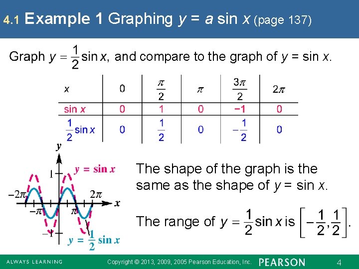
4. 1 Example 1 Graphing y = a sin x (page 137) and compare to the graph of y = sin x. The shape of the graph is the same as the shape of y = sin x. The range of Copyright © 2013, 2009, 2005 Pearson Education, Inc. is 4

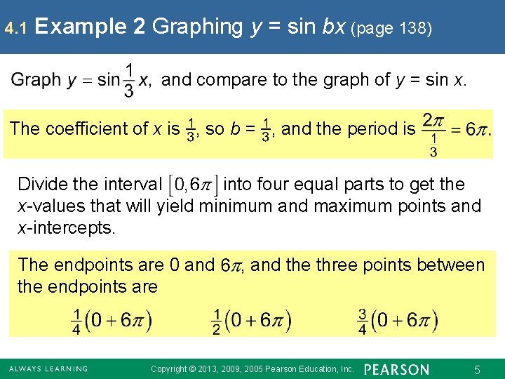
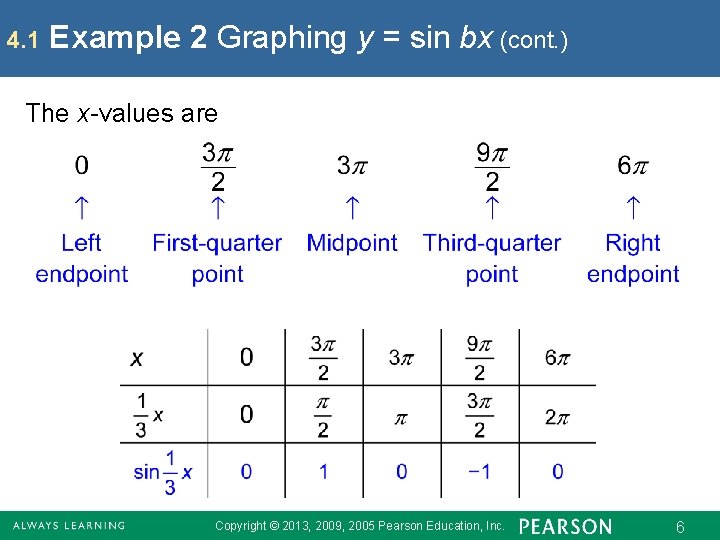
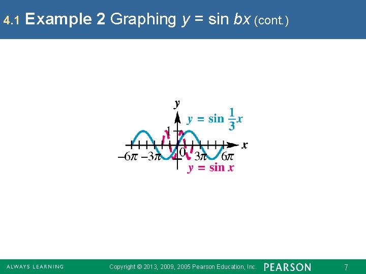
4. 1 Example 2 Graphing y = sin bx (page 138) and compare to the graph of y = sin x. The coefficient of x is , so b = , and the period is Divide the interval into four equal parts to get the x-values that will yield minimum and maximum points and x-intercepts. The endpoints are 0 and the endpoints are , and the three points between Copyright © 2013, 2009, 2005 Pearson Education, Inc. 5

4. 1 Example 2 Graphing y = sin bx (cont. ) The x-values are Copyright © 2013, 2009, 2005 Pearson Education, Inc. 6

4. 1 Example 2 Graphing y = sin bx (cont. ) Copyright © 2013, 2009, 2005 Pearson Education, Inc. 7

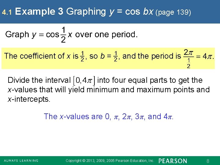
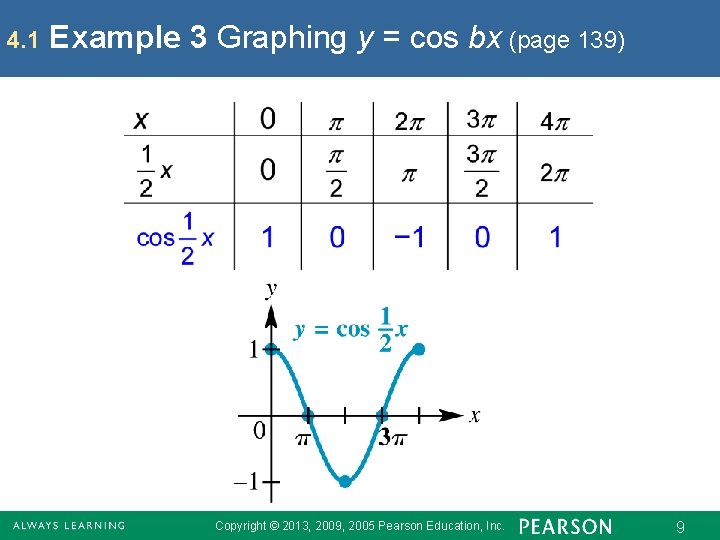
4. 1 Example 3 Graphing y = cos bx (page 139) The coefficient of x is , so b = , and the period is Divide the interval into four equal parts to get the x-values that will yield minimum and maximum points and x-intercepts. The x-values are 0, π, 2π, 3π, and 4π. Copyright © 2013, 2009, 2005 Pearson Education, Inc. 8

4. 1 Example 3 Graphing y = cos bx (page 139) Copyright © 2013, 2009, 2005 Pearson Education, Inc. 9

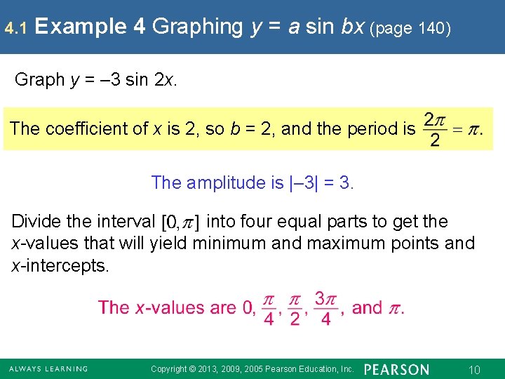
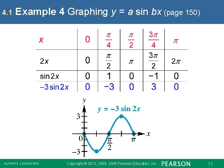
4. 1 Example 4 Graphing y = a sin bx (page 140) Graph y = – 3 sin 2 x. The coefficient of x is 2, so b = 2, and the period is The amplitude is |– 3| = 3. Divide the interval into four equal parts to get the x-values that will yield minimum and maximum points and x-intercepts. Copyright © 2013, 2009, 2005 Pearson Education, Inc. 10

4. 1 Example 4 Graphing y = a sin bx (page 150) Copyright © 2013, 2009, 2005 Pearson Education, Inc. 11

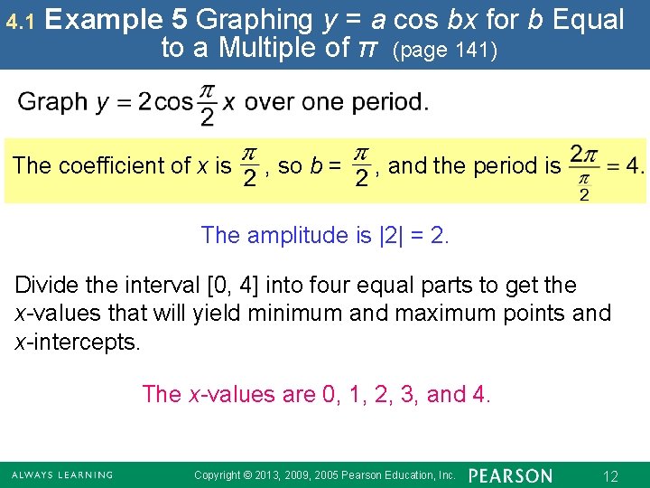
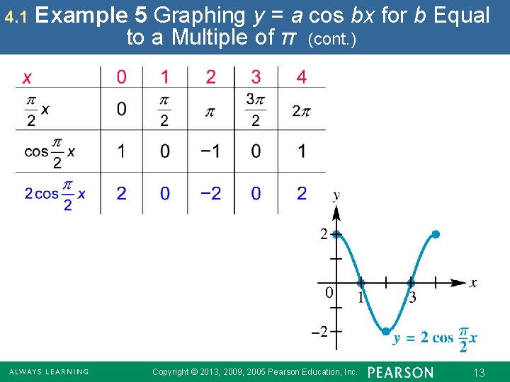
4. 1 Example 5 Graphing y = a cos bx for b Equal to a Multiple of π (page 141) The coefficient of x is , so b = , and the period is The amplitude is |2| = 2. Divide the interval [0, 4] into four equal parts to get the x-values that will yield minimum and maximum points and x-intercepts. The x-values are 0, 1, 2, 3, and 4. Copyright © 2013, 2009, 2005 Pearson Education, Inc. 12

4. 1 Example 5 Graphing y = a cos bx for b Equal to a Multiple of π (cont. ) Copyright © 2013, 2009, 2005 Pearson Education, Inc. 13

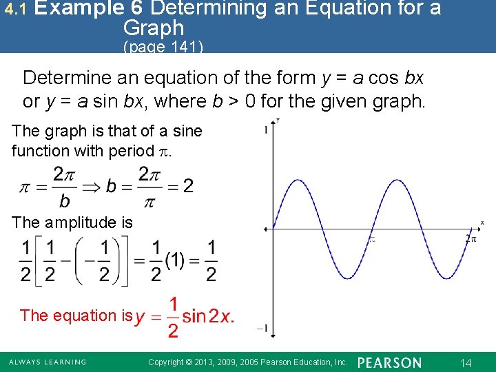
4. 1 Example 6 Determining an Equation for a Graph (page 141) Determine an equation of the form y = a cos bx or y = a sin bx, where b > 0 for the given graph. The graph is that of a sine function with period . The amplitude is The equation is Copyright © 2013, 2009, 2005 Pearson Education, Inc. 14

4. 2 Translations of the Graphs of the Sine and Cosine Functions Horizontal Translations ▪ Vertical Translations ▪ Combinations of Translations ▪ Determining a Trigonometric Model Using Curve Fitting Copyright © 2013, 2009, 2005 Pearson Education, Inc. 15

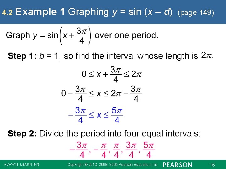
4. 2 Example 1 Graphing y = sin (x – d) (page 149) Step 1: b = 1, so find the interval whose length is Step 2: Divide the period into four equal intervals: Copyright © 2013, 2009, 2005 Pearson Education, Inc. 16

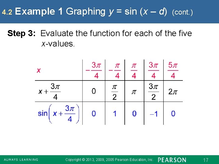
4. 2 Example 1 Graphing y = sin (x – d) (cont. ) Step 3: Evaluate the function for each of the five x-values. Copyright © 2013, 2009, 2005 Pearson Education, Inc. 17

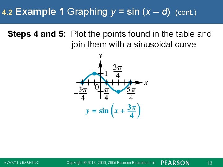
4. 2 Example 1 Graphing y = sin (x – d) (cont. ) Steps 4 and 5: Plot the points found in the table and join them with a sinusoidal curve. Copyright © 2013, 2009, 2005 Pearson Education, Inc. 18

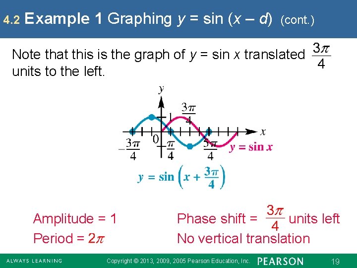
4. 2 Example 1 Graphing y = sin (x – d) (cont. ) Note that this is the graph of y = sin x translated units to the left. Amplitude = 1 Period = Phase shift = units left No vertical translation Copyright © 2013, 2009, 2005 Pearson Education, Inc. 19

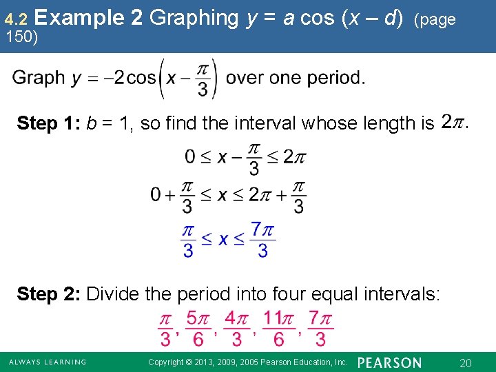
4. 2 Example 150) 2 Graphing y = a cos (x – d) (page Step 1: b = 1, so find the interval whose length is Step 2: Divide the period into four equal intervals: Copyright © 2013, 2009, 2005 Pearson Education, Inc. 20

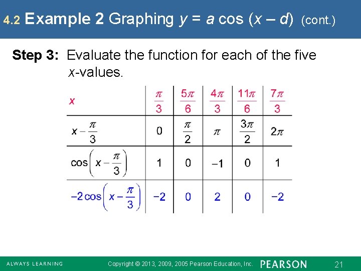
4. 2 Example 2 Graphing y = a cos (x – d) (cont. ) Step 3: Evaluate the function for each of the five x-values. Copyright © 2013, 2009, 2005 Pearson Education, Inc. 21

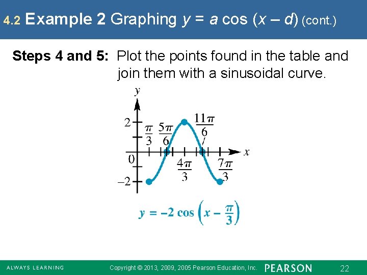
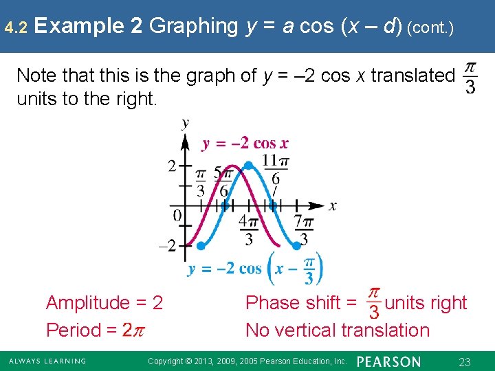
4. 2 Example 2 Graphing y = a cos (x – d) (cont. ) Steps 4 and 5: Plot the points found in the table and join them with a sinusoidal curve. Copyright © 2013, 2009, 2005 Pearson Education, Inc. 22

4. 2 Example 2 Graphing y = a cos (x – d) (cont. ) Note that this is the graph of y = – 2 cos x translated units to the right. Amplitude = 2 Period = Phase shift = units right No vertical translation Copyright © 2013, 2009, 2005 Pearson Education, Inc. 23

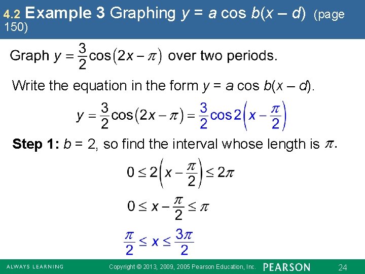
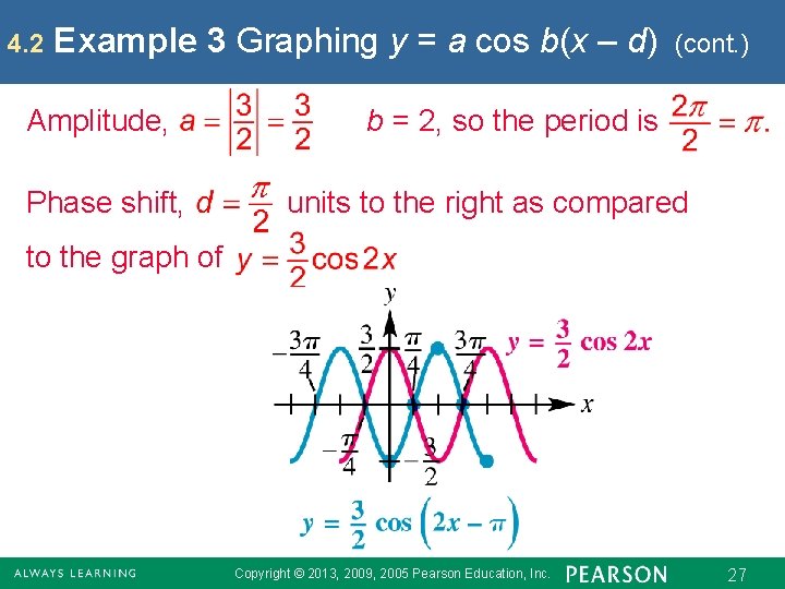
4. 2 Example 150) 3 Graphing y = a cos b(x – d) (page Write the equation in the form y = a cos b(x – d). Step 1: b = 2, so find the interval whose length is Copyright © 2013, 2009, 2005 Pearson Education, Inc. 24

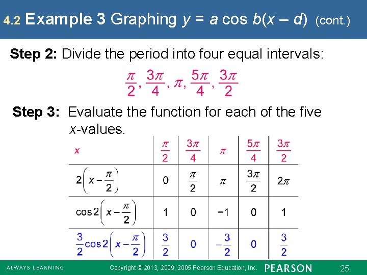
4. 2 Example 3 Graphing y = a cos b(x – d) (cont. ) Step 2: Divide the period into four equal intervals: Step 3: Evaluate the function for each of the five x-values. Copyright © 2013, 2009, 2005 Pearson Education, Inc. 25

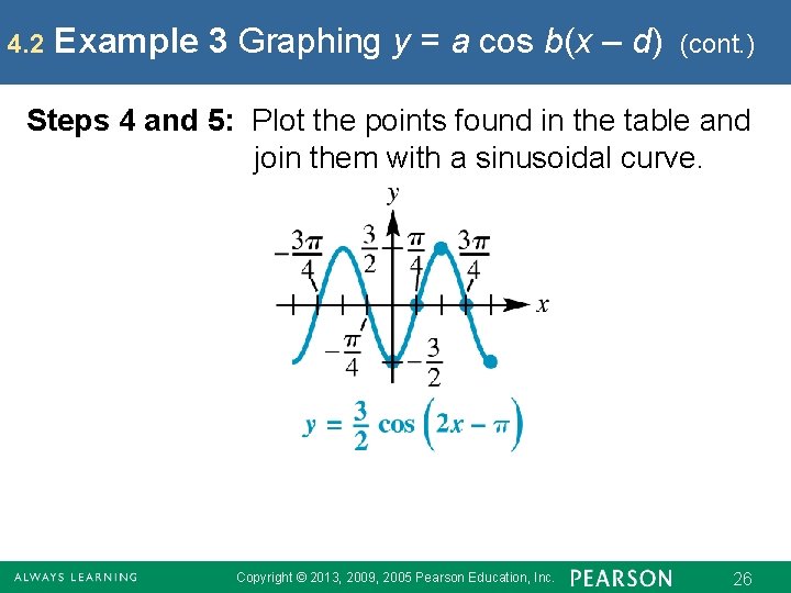
4. 2 Example 3 Graphing y = a cos b(x – d) (cont. ) Steps 4 and 5: Plot the points found in the table and join them with a sinusoidal curve. Copyright © 2013, 2009, 2005 Pearson Education, Inc. 26

4. 2 Example 3 Graphing y = a cos b(x – d) Amplitude, Phase shift, (cont. ) b = 2, so the period is units to the right as compared to the graph of Copyright © 2013, 2009, 2005 Pearson Education, Inc. 27

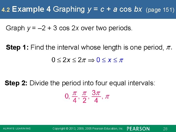
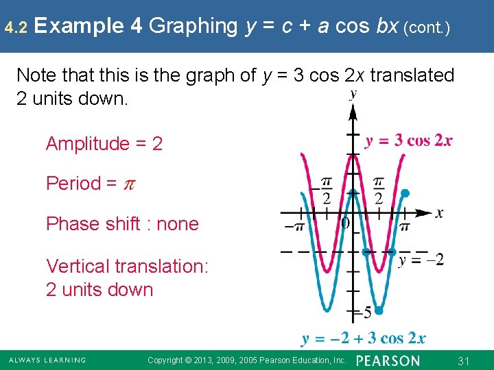
4. 2 Example 4 Graphing y = c + a cos bx (page 151) Graph y = – 2 + 3 cos 2 x over two periods. Step 1: Find the interval whose length is one period, Step 2: Divide the period into four equal intervals: Copyright © 2013, 2009, 2005 Pearson Education, Inc. 28

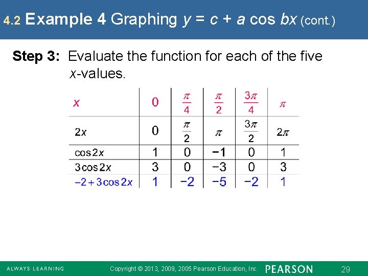
4. 2 Example 4 Graphing y = c + a cos bx (cont. ) Step 3: Evaluate the function for each of the five x-values. Copyright © 2013, 2009, 2005 Pearson Education, Inc. 29

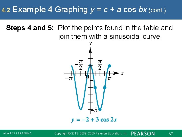
4. 2 Example 4 Graphing y = c + a cos bx (cont. ) Steps 4 and 5: Plot the points found in the table and join them with a sinusoidal curve. Copyright © 2013, 2009, 2005 Pearson Education, Inc. 30

4. 2 Example 4 Graphing y = c + a cos bx (cont. ) Note that this is the graph of y = 3 cos 2 x translated 2 units down. Amplitude = 2 Period = Phase shift : none Vertical translation: 2 units down Copyright © 2013, 2009, 2005 Pearson Education, Inc. 31

4. 3 Graphs of the Tangent and Cotangent Functions Graph of the Tangent Function ▪ Graph of the Cotangent Function ▪ Graphing Techniques Copyright © 2013, 2009, 2005 Pearson Education, Inc. 32

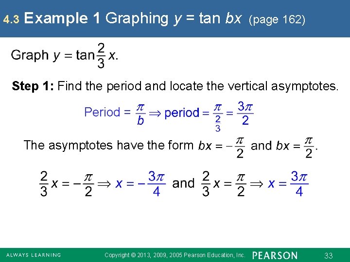
4. 3 Example 1 Graphing y = tan bx (page 162) Step 1: Find the period and locate the vertical asymptotes. Period = The asymptotes have the form Copyright © 2013, 2009, 2005 Pearson Education, Inc. 33

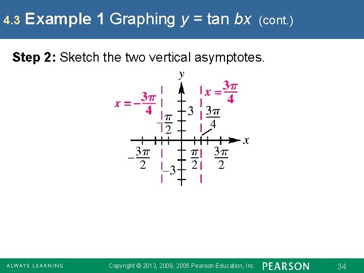
4. 3 Example 1 Graphing y = tan bx (cont. ) Step 2: Sketch the two vertical asymptotes. Copyright © 2013, 2009, 2005 Pearson Education, Inc. 34

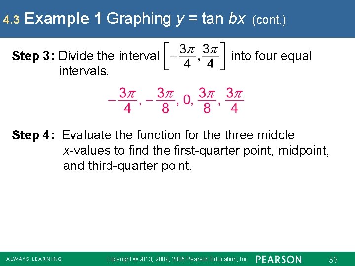
4. 3 Example 1 Graphing y = tan bx Step 3: Divide the intervals. (cont. ) into four equal Step 4: Evaluate the function for the three middle x-values to find the first-quarter point, midpoint, and third-quarter point. Copyright © 2013, 2009, 2005 Pearson Education, Inc. 35

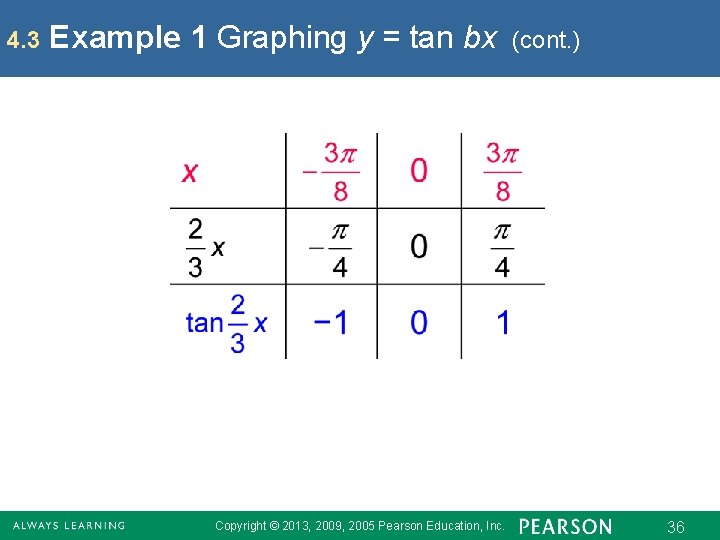
4. 3 Example 1 Graphing y = tan bx Copyright © 2013, 2009, 2005 Pearson Education, Inc. (cont. ) 36

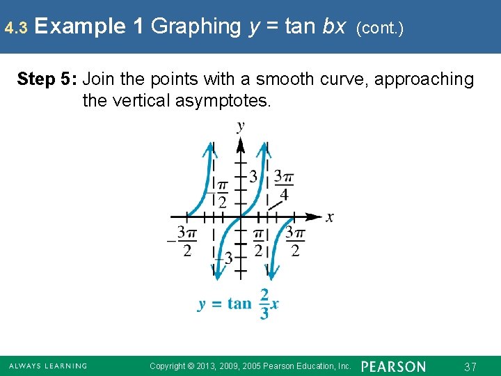
4. 3 Example 1 Graphing y = tan bx (cont. ) Step 5: Join the points with a smooth curve, approaching the vertical asymptotes. Copyright © 2013, 2009, 2005 Pearson Education, Inc. 37

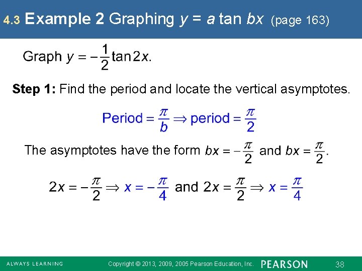
4. 3 Example 2 Graphing y = a tan bx (page 163) Step 1: Find the period and locate the vertical asymptotes. The asymptotes have the form Copyright © 2013, 2009, 2005 Pearson Education, Inc. 38

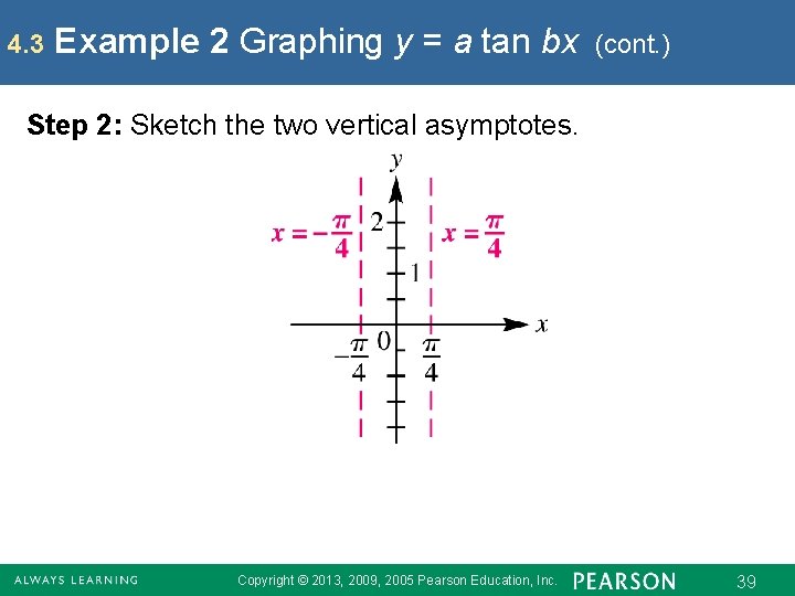
4. 3 Example 2 Graphing y = a tan bx (cont. ) Step 2: Sketch the two vertical asymptotes. Copyright © 2013, 2009, 2005 Pearson Education, Inc. 39

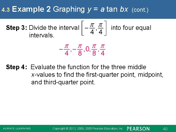
4. 3 Example 2 Graphing y = a tan bx Step 3: Divide the intervals. (cont. ) into four equal Step 4: Evaluate the function for the three middle x-values to find the first-quarter point, midpoint, and third-quarter point. Copyright © 2013, 2009, 2005 Pearson Education, Inc. 40

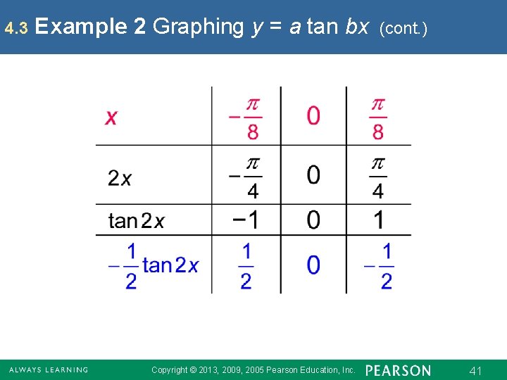
4. 3 Example 2 Graphing y = a tan bx Copyright © 2013, 2009, 2005 Pearson Education, Inc. (cont. ) 41

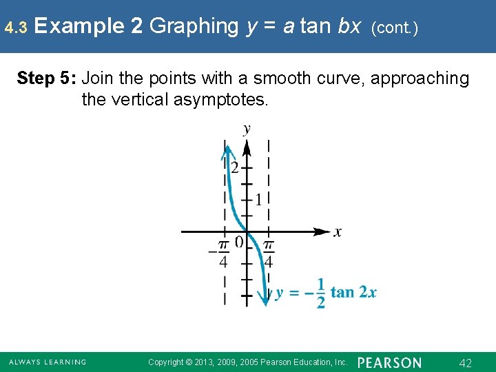
4. 3 Example 2 Graphing y = a tan bx (cont. ) Step 5: Join the points with a smooth curve, approaching the vertical asymptotes. Copyright © 2013, 2009, 2005 Pearson Education, Inc. 42

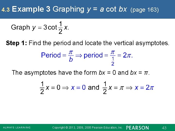
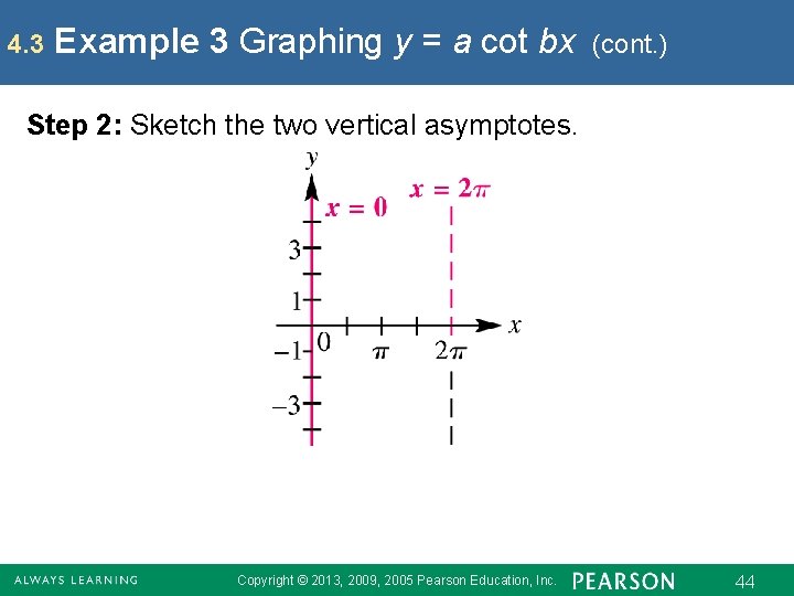
4. 3 Example 3 Graphing y = a cot bx (page 163) Step 1: Find the period and locate the vertical asymptotes. The asymptotes have the form bx = 0 and bx = π. Copyright © 2013, 2009, 2005 Pearson Education, Inc. 43

4. 3 Example 3 Graphing y = a cot bx (cont. ) Step 2: Sketch the two vertical asymptotes. Copyright © 2013, 2009, 2005 Pearson Education, Inc. 44

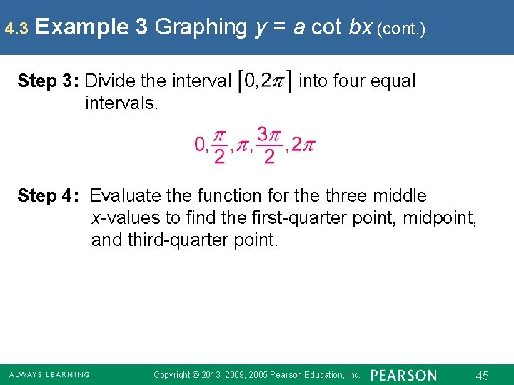
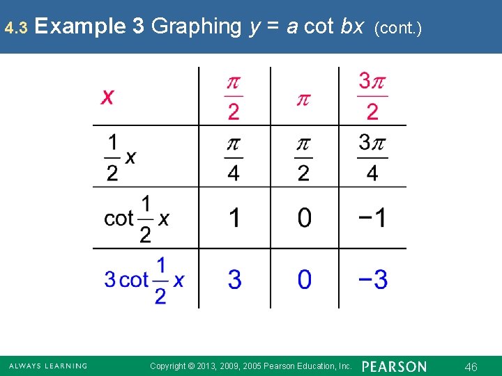
4. 3 Example 3 Graphing y = a cot bx (cont. ) Step 3: Divide the intervals. into four equal Step 4: Evaluate the function for the three middle x-values to find the first-quarter point, midpoint, and third-quarter point. Copyright © 2013, 2009, 2005 Pearson Education, Inc. 45

4. 3 Example 3 Graphing y = a cot bx Copyright © 2013, 2009, 2005 Pearson Education, Inc. (cont. ) 46

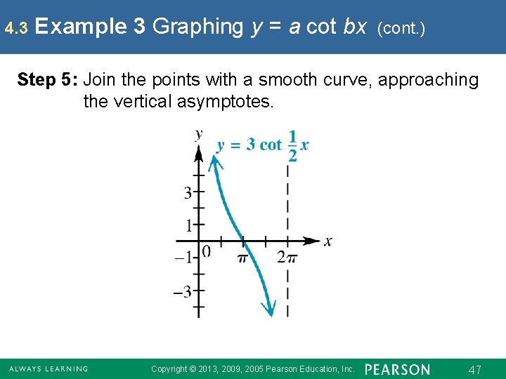
4. 3 Example 3 Graphing y = a cot bx (cont. ) Step 5: Join the points with a smooth curve, approaching the vertical asymptotes. Copyright © 2013, 2009, 2005 Pearson Education, Inc. 47

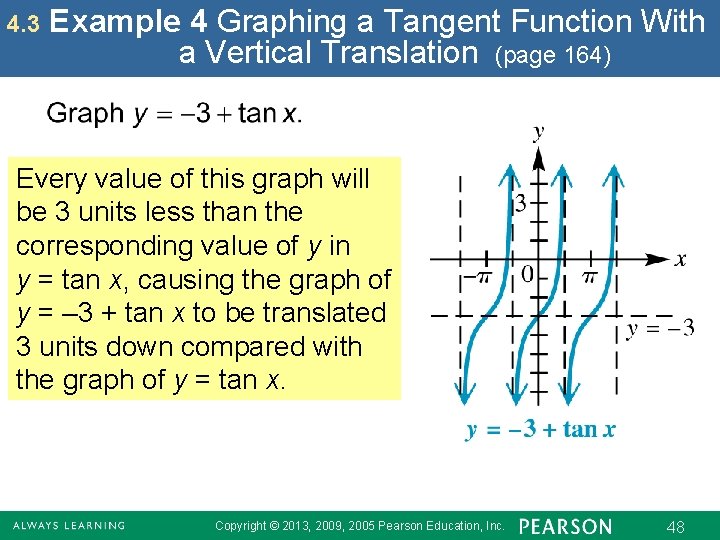
4. 3 Example 4 Graphing a Tangent Function With a Vertical Translation (page 164) Every value of this graph will be 3 units less than the corresponding value of y in y = tan x, causing the graph of y = – 3 + tan x to be translated 3 units down compared with the graph of y = tan x. Copyright © 2013, 2009, 2005 Pearson Education, Inc. 48

4. 4 Graphs of the Secant and Cosecant Functions Graph of the Secant Function ▪ Graph of the Cosecant Function ▪ Graphing Techniques ▪ Addition of Ordinates ▪ Connecting Graphs with Equations Copyright © 2013, 2009, 2005 Pearson Education, Inc. 49

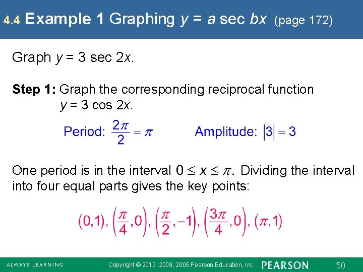
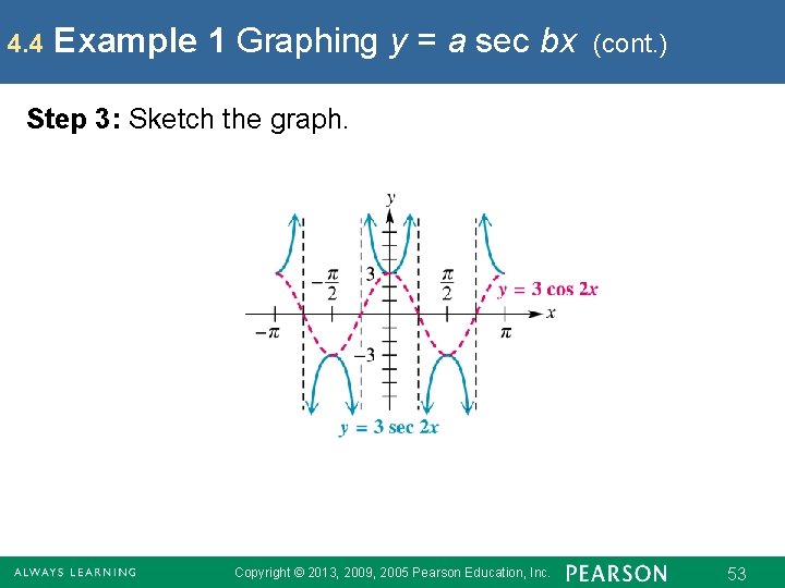
4. 4 Example 1 Graphing y = a sec bx (page 172) Graph y = 3 sec 2 x. Step 1: Graph the corresponding reciprocal function y = 3 cos 2 x. One period is in the interval Dividing the interval into four equal parts gives the key points: Copyright © 2013, 2009, 2005 Pearson Education, Inc. 50

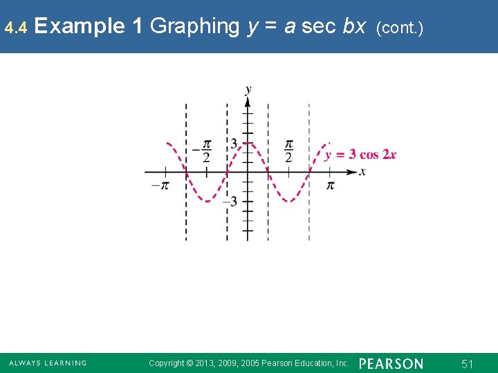
4. 4 Example 1 Graphing y = a sec bx Copyright © 2013, 2009, 2005 Pearson Education, Inc. (cont. ) 51

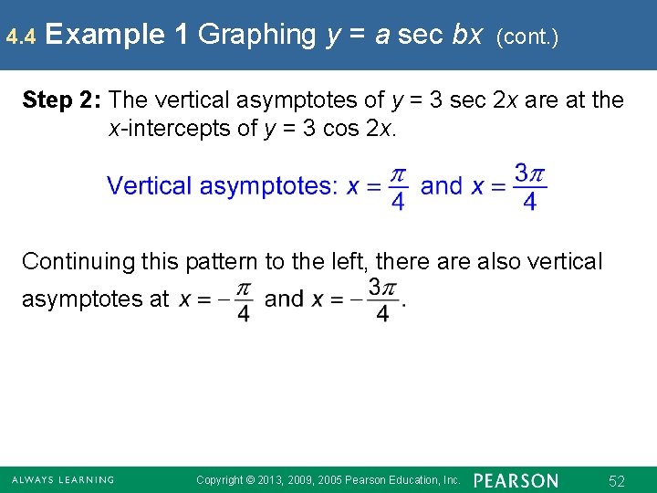
4. 4 Example 1 Graphing y = a sec bx (cont. ) Step 2: The vertical asymptotes of y = 3 sec 2 x are at the x-intercepts of y = 3 cos 2 x. Continuing this pattern to the left, there also vertical asymptotes at Copyright © 2013, 2009, 2005 Pearson Education, Inc. 52

4. 4 Example 1 Graphing y = a sec bx (cont. ) Step 3: Sketch the graph. Copyright © 2013, 2009, 2005 Pearson Education, Inc. 53

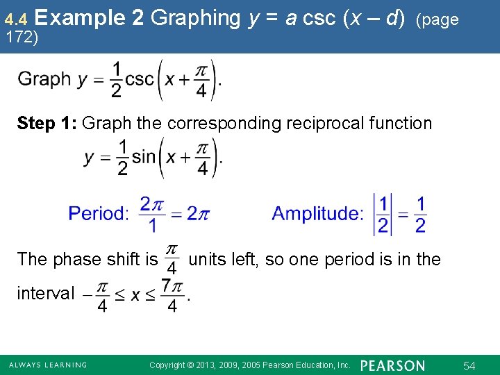
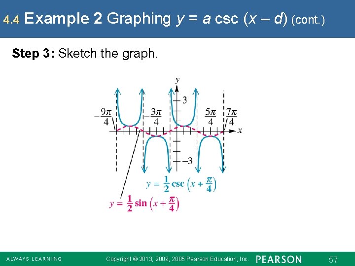
4. 4 Example 172) 2 Graphing y = a csc (x – d) (page Step 1: Graph the corresponding reciprocal function The phase shift is units left, so one period is in the interval Copyright © 2013, 2009, 2005 Pearson Education, Inc. 54

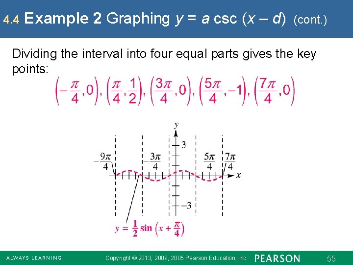
4. 4 Example 2 Graphing y = a csc (x – d) (cont. ) Dividing the interval into four equal parts gives the key points: Copyright © 2013, 2009, 2005 Pearson Education, Inc. 55

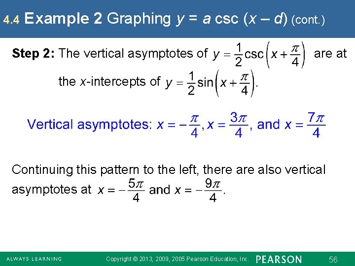
4. 4 Example 2 Graphing y = a csc (x – d) (cont. ) Step 2: The vertical asymptotes of are at the x-intercepts of Continuing this pattern to the left, there also vertical asymptotes at Copyright © 2013, 2009, 2005 Pearson Education, Inc. 56

4. 4 Example 2 Graphing y = a csc (x – d) (cont. ) Step 3: Sketch the graph. Copyright © 2013, 2009, 2005 Pearson Education, Inc. 57

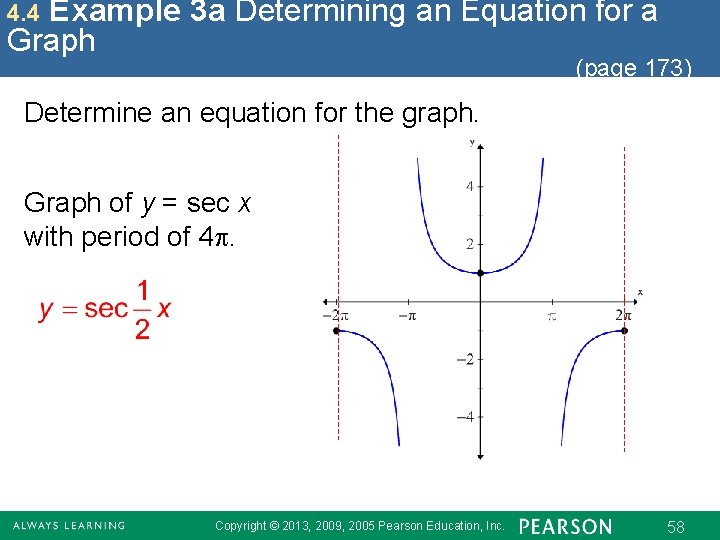
Example 3 a Determining an Equation for a Graph 4. 4 (page 173) Determine an equation for the graph. Graph of y = sec x with period of 4. Copyright © 2013, 2009, 2005 Pearson Education, Inc. 58

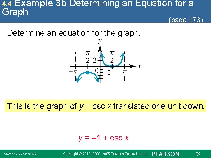
Example 3 b Determining an Equation for a Graph 4. 4 (page 173) Determine an equation for the graph. This is the graph of y = csc x translated one unit down. y = – 1 + csc x Copyright © 2013, 2009, 2005 Pearson Education, Inc. 59