4 Associated Legendre Equation Associated Legendre Eq Let

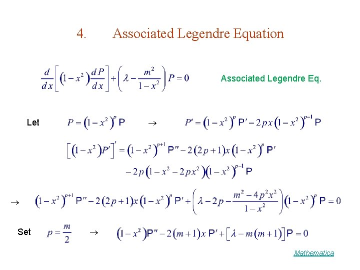
4. Associated Legendre Equation Associated Legendre Eq. Let Set Mathematica

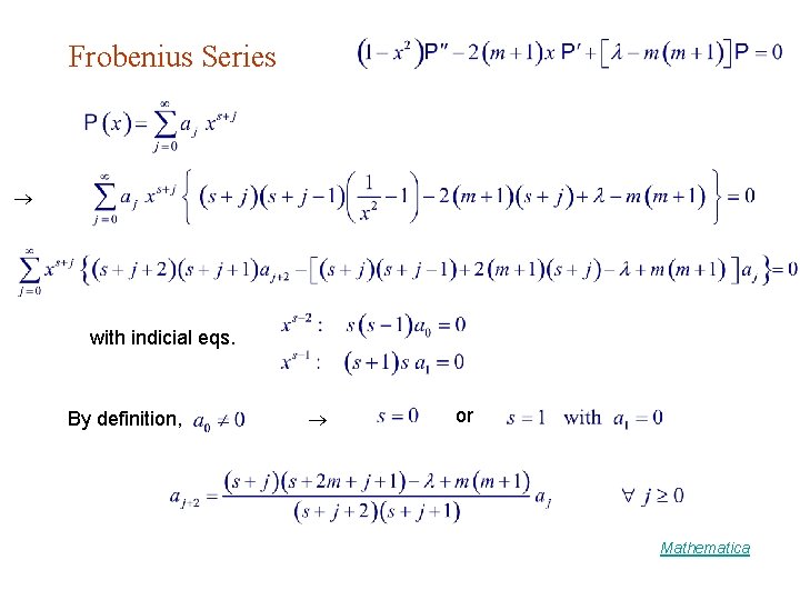
Frobenius Series with indicial eqs. By definition, or Mathematica

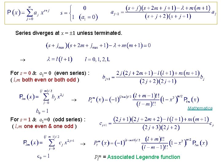
Series diverges at x = 1 unless terminated. For s = 0 & a 1= 0 (even series) : ( l, m both even or both odd ) Mathematica For s = 1 & a 1=0 (odd series) : ( l, m one even & one odd ) Plm = Associated Legendre function

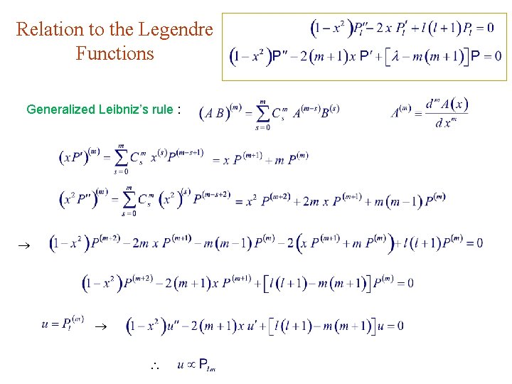
Relation to the Legendre Functions Generalized Leibniz’s rule :

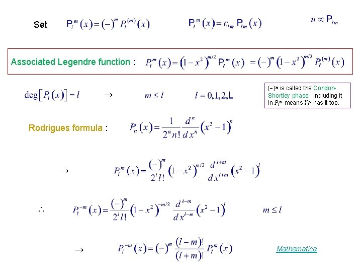
Set Associated Legendre function : ( )m is called the Condon. Shortley phase. Including it in Plm means Ylm has it too. Rodrigues formula : Mathematica

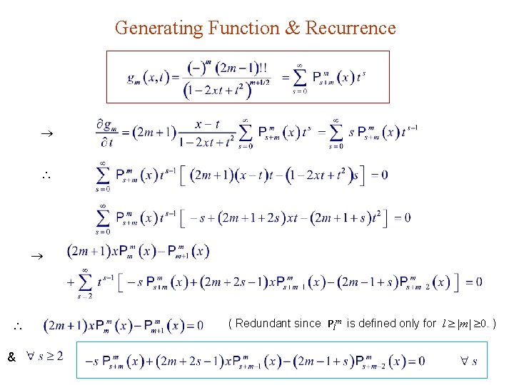
Generating Function & Recurrence & ( Redundant since Plm is defined only for l |m| 0. )

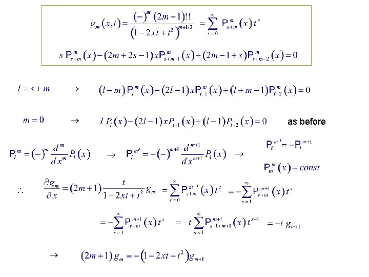
as before

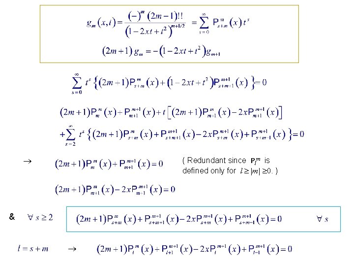
( Redundant since Plm is defined only for l |m| 0. ) &

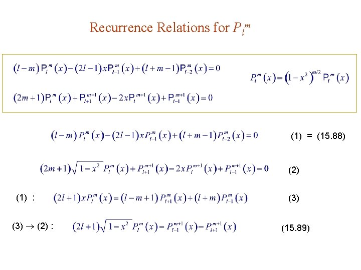
Recurrence Relations for Plm (1) = (15. 88) (2) (1) : (3) (2) : (3) (15. 89)

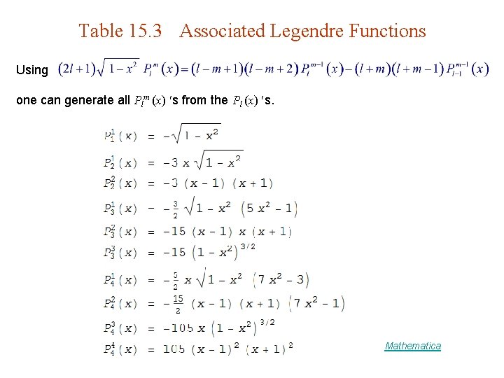
Table 15. 3 Associated Legendre Functions Using one can generate all Plm (x) s from the Pl (x) s. Mathematica

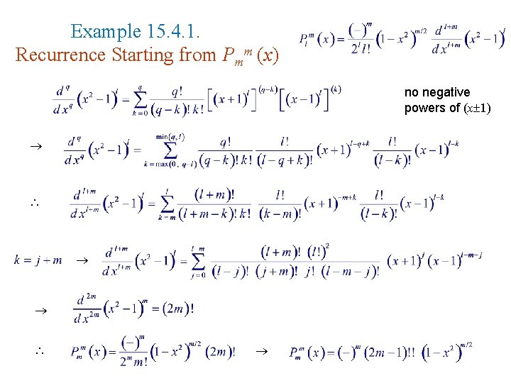
Example 15. 4. 1. Recurrence Starting from Pmm (x) no negative powers of (x 1)

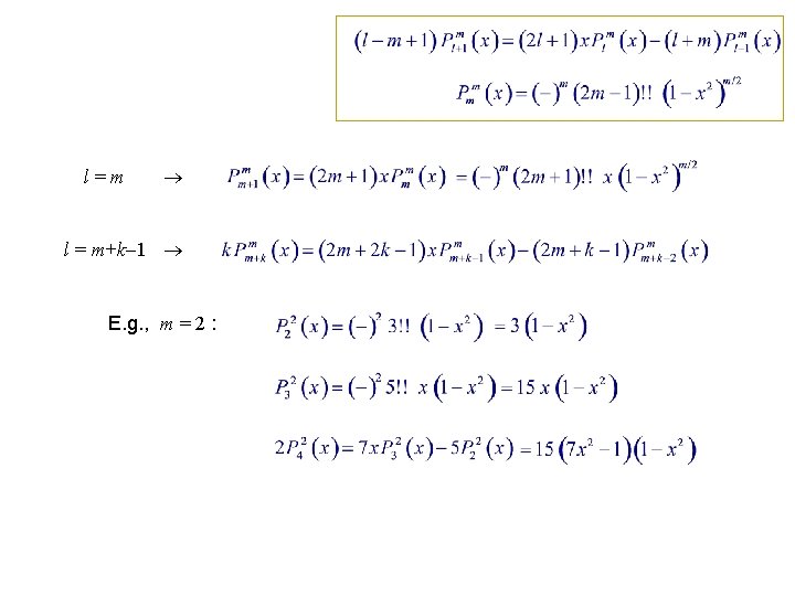
l=m l = m+k 1 E. g. , m = 2 :

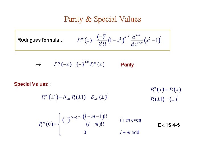
Parity & Special Values Rodrigues formula : Parity Special Values : Ex. 15. 4 -5

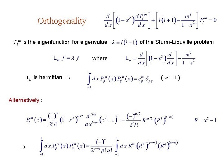
Orthogonality Plm is the eigenfunction for eigenvalue of the Sturm-Liouville problem where Lm is hermitian Alternatively : (w=1)

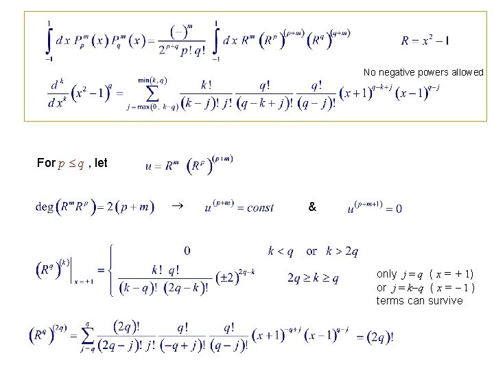
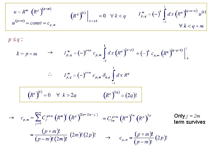
No negative powers allowed For p q , let & only j = q ( x = + 1) or j = k q ( x = 1 ) terms can survive

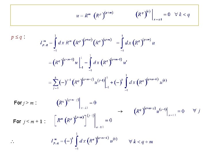
p q: For j > m : For j < m + 1 :

p q: Only j = 2 m term survives

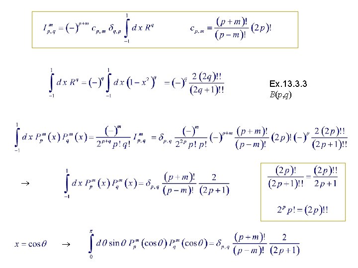
Ex. 13. 3. 3 B(p, q)

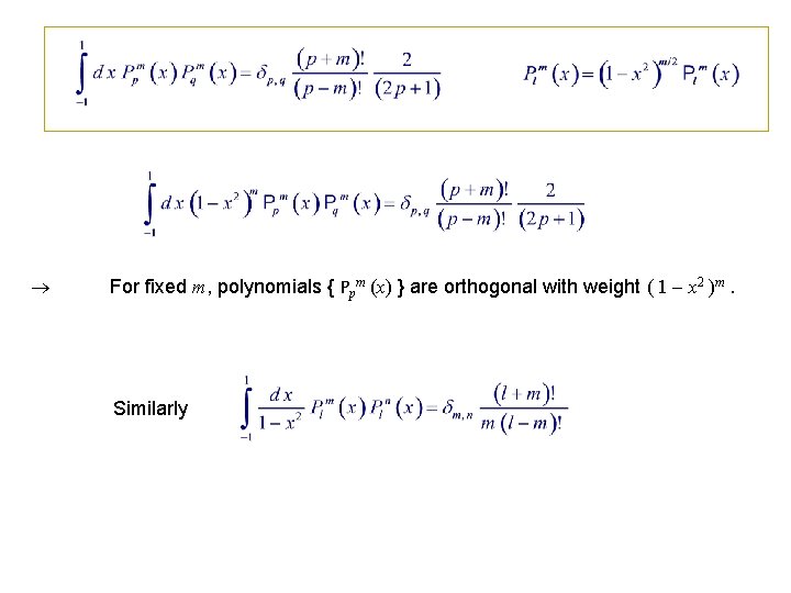
For fixed m, polynomials { Ppm (x) } are orthogonal with weight ( 1 x 2 )m. Similarly

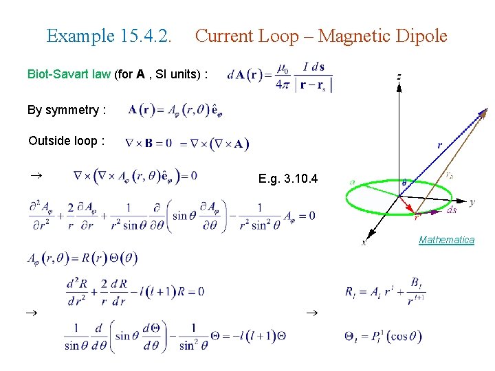
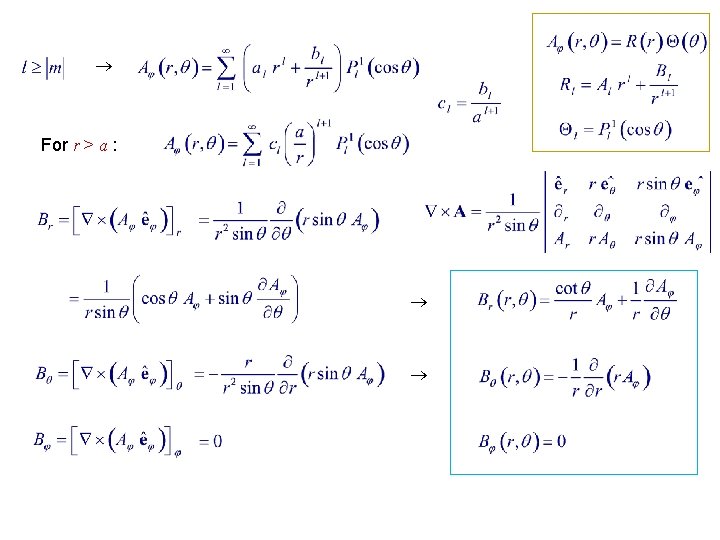
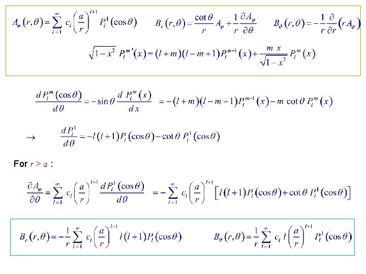
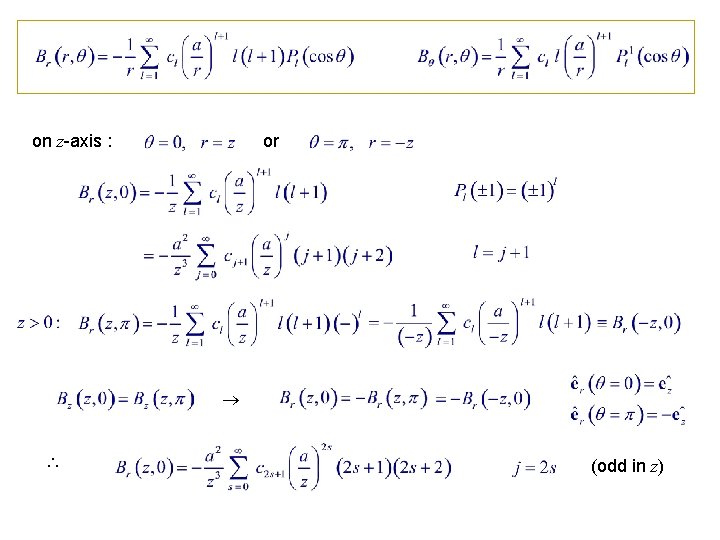
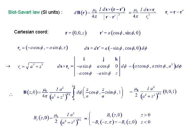
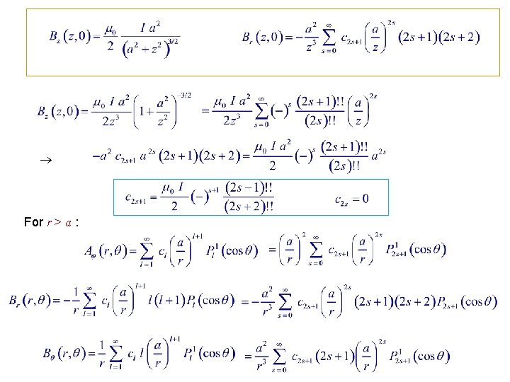
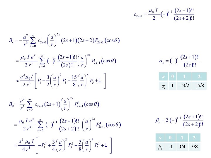
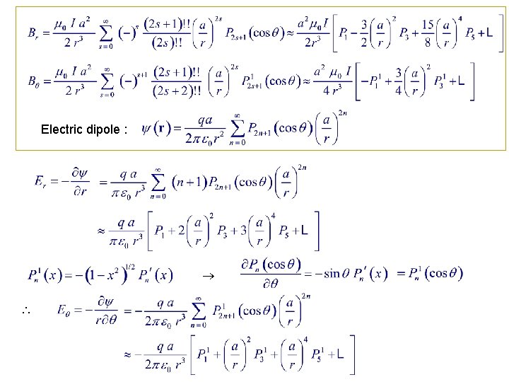
Example 15. 4. 2. Current Loop – Magnetic Dipole Biot-Savart law (for A , SI units) : By symmetry : Outside loop : E. g. 3. 10. 4 Mathematica

For r > a :

For r > a :

on z-axis : or (odd in z)

Biot-Savart law (SI units) : Cartesian coord:

For r > a :

s 0 1 2 s 1 3/2 15/8 s 0 1 2 s 1 3/4 5/8

Electric dipole :

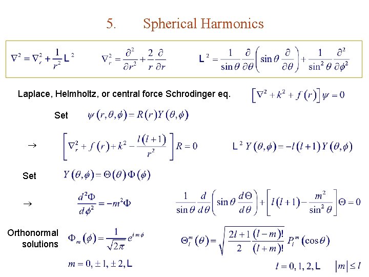
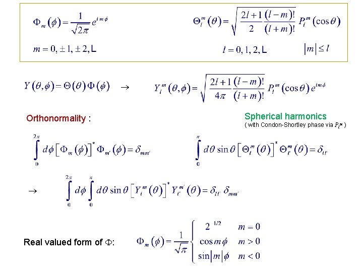
5. Spherical Harmonics Laplace, Helmholtz, or central force Schrodinger eq. Set Orthonormal solutions

Orthonormality : Real valued form of : Spherical harmonics ( with Condon-Shortley phase via Plm )

Fig. 15. 12. Shapes of [ Re Ylm ( , ) ]2 Surfaces are given by Y 00 Y 10 Y 20 Y 11 Y 22 Y 21 Mathematica Y 30 Y 31 Y 32 Y 33

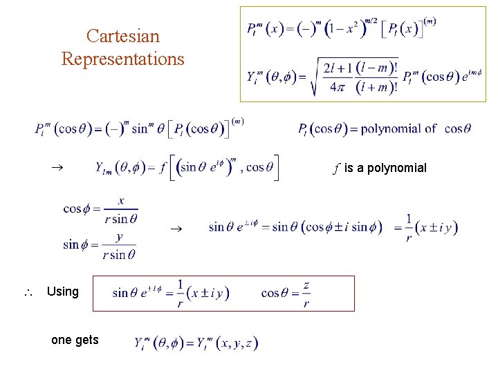
Cartesian Representations f is a polynomial Using one gets

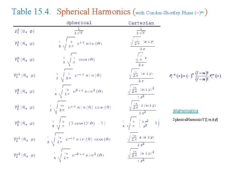
Table 15. 4. Spherical Harmonics (with Condon-Shortley Phase ( ) ) m Mathematica Spherical. Harmonic. Y[l, m, , ] Mathematica

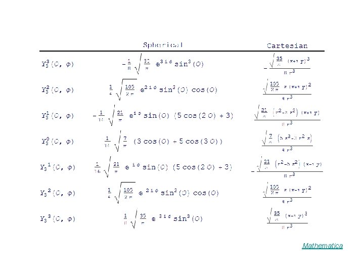
Mathematica

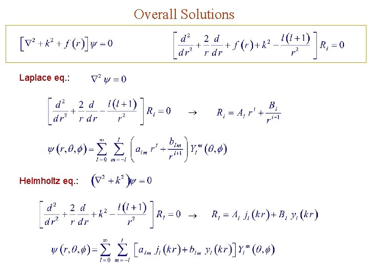
Overall Solutions Laplace eq. : Helmholtz eq. :

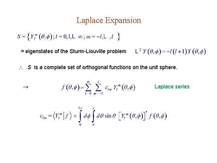
Laplace Expansion = eigenstates of the Sturm-Liouville problem S is a complete set of orthogonal functions on the unit sphere. Laplace series

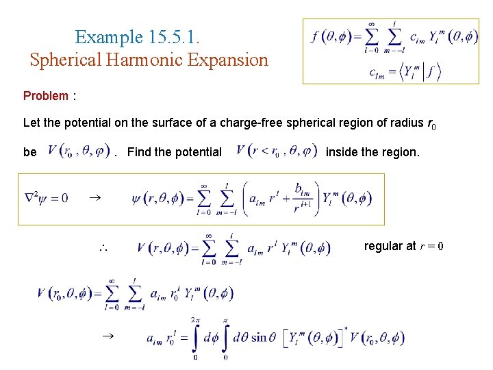
Example 15. 5. 1. Spherical Harmonic Expansion Problem : Let the potential on the surface of a charge-free spherical region of radius r 0 be . Find the potential inside the region. regular at r = 0

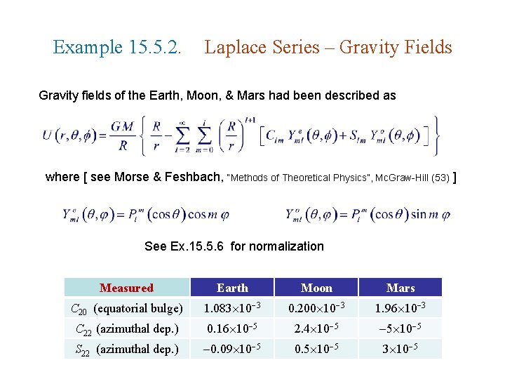
Example 15. 5. 2. Laplace Series – Gravity Fields Gravity fields of the Earth, Moon, & Mars had been described as where [ see Morse & Feshbach, “Methods of Theoretical Physics”, Mc. Graw-Hill (53) ] See Ex. 15. 5. 6 for normalization Measured Earth Moon Mars C 20 (equatorial bulge) 1. 083 10 3 0. 200 10 3 1. 96 10 3 C 22 (azimuthal dep. ) 0. 16 10 5 2. 4 10 5 5 10 5 S 22 (azimuthal dep. ) 0. 09 10 5 0. 5 10 5 3 10 5

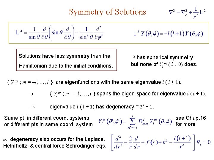
Symmetry of Solutions have less symmetry than the Hamiltonian due to the initial conditions. L 2 has spherical symmetry but none of Yl m ( l 0) does. { Yl m ; m = l, …, l } are eigenfunctions with the same eigenvalue l ( l + 1). { Yl m ; m = l, …, l } spans the eigen-space for eigenvalue l ( l + 1) has degeneracy = 2 l + 1. Same pt. in different coord. systems or different pts in same coord. system m degeneracy also occurs for the Laplace, Helmholtz, & central force Schrodinger eqs. see Chap. 16 for more

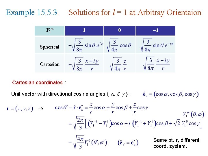
Example 15. 5. 3. Y 1 m Solutions for l = 1 at Arbitray Orientaion 1 0 1 Spherical Cartesian coordinates : Unit vector with directional cosine angles { , , } : Same pt. r, different coord. system.

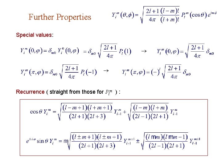
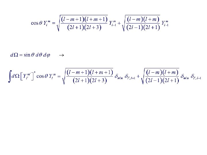
Further Properties Special values: Recurrence ( straight from those for Plm ) :

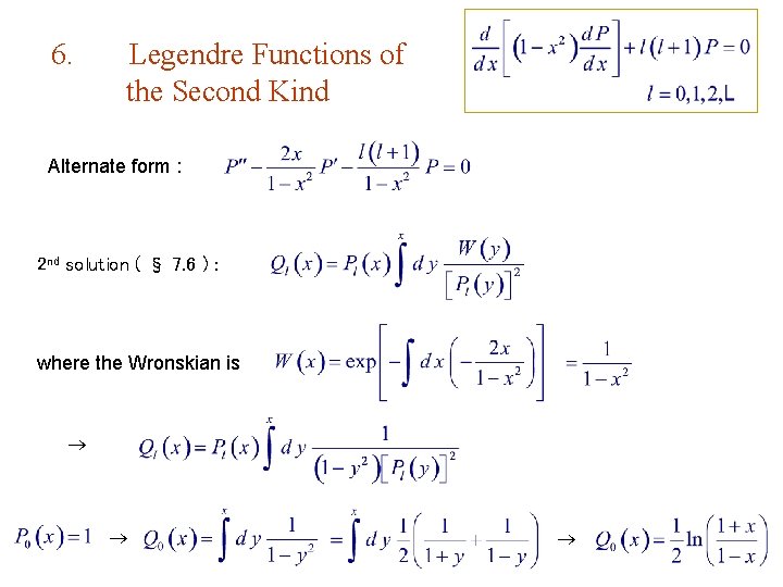
6. Legendre Functions of the Second Kind Alternate form : 2 nd solution ( § 7. 6 ) : where the Wronskian is

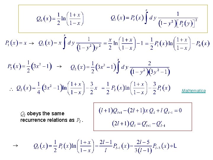
Mathematica Ql obeys the same recurrence relations as Pl.

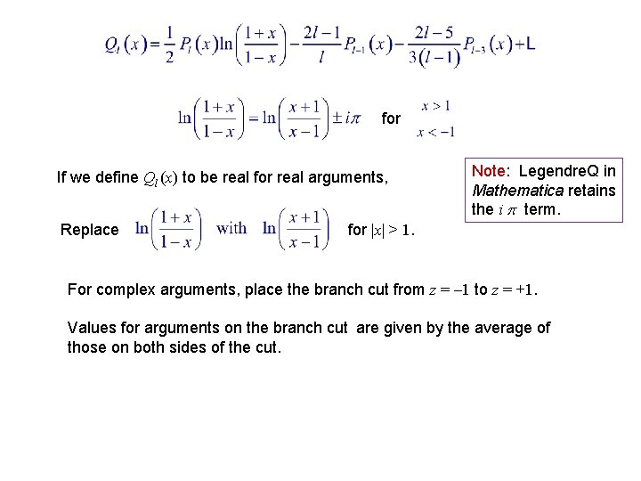
for If we define Ql (x) to be real for real arguments, Replace Note: Legendre. Q in Mathematica retains the i term. for |x| > 1. For complex arguments, place the branch cut from z = 1 to z = +1. Values for arguments on the branch cut are given by the average of those on both sides of the cut.

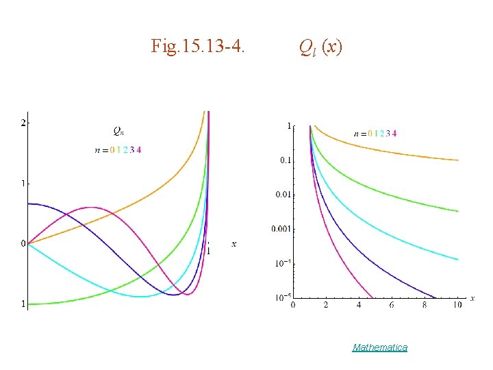
Fig. 15. 13 -4. Ql (x) Mathematica

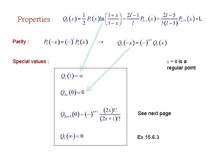
Properties Parity : x = 0 is a regular point Special values : See next page Ex. 15. 6. 3

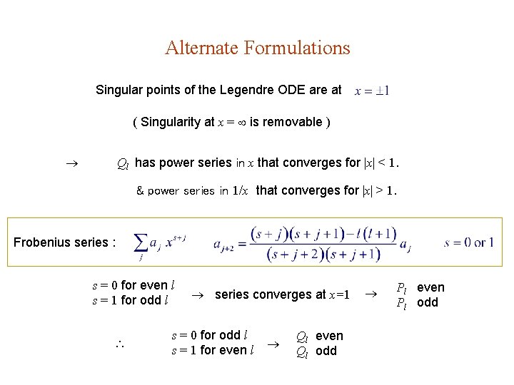
Alternate Formulations Singular points of the Legendre ODE are at ( Singularity at x = is removable ) Ql has power series in x that converges for |x| < 1. & power series in 1/x that converges for |x| > 1. Frobenius series : s = 0 for even l s = 1 for odd l series converges at x=1 s = 0 for odd l s = 1 for even l Ql even Ql odd Pl even Pl odd

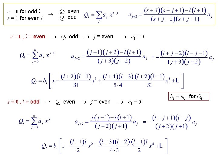
s = 0 for odd l s = 1 for even l s = 1 , l = even s = 0 , l = odd Ql even Ql odd Ql even j = even a 1 = 0 bl = a 0 for Ql

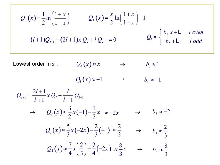
Lowest order in x :

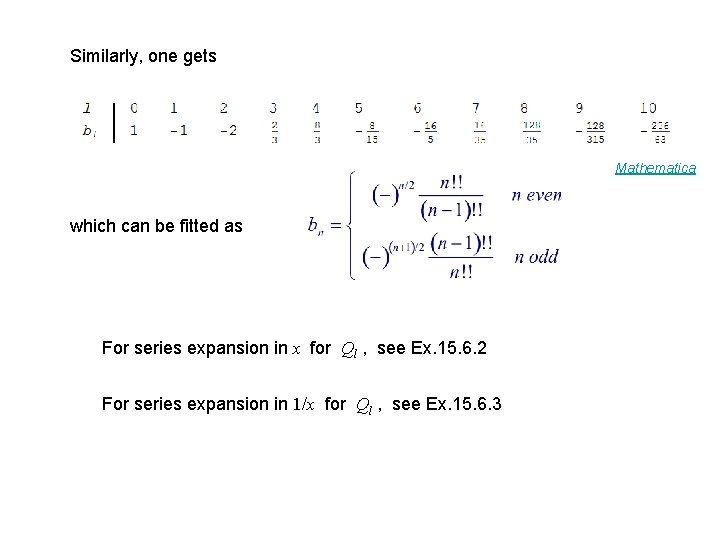
Similarly, one gets Mathematica which can be fitted as For series expansion in x for Ql , see Ex. 15. 6. 2 For series expansion in 1/x for Ql , see Ex. 15. 6. 3