4 5 Linear Approximations and Differentials Mysterious radiation

4. 5: Linear Approximations and Differentials

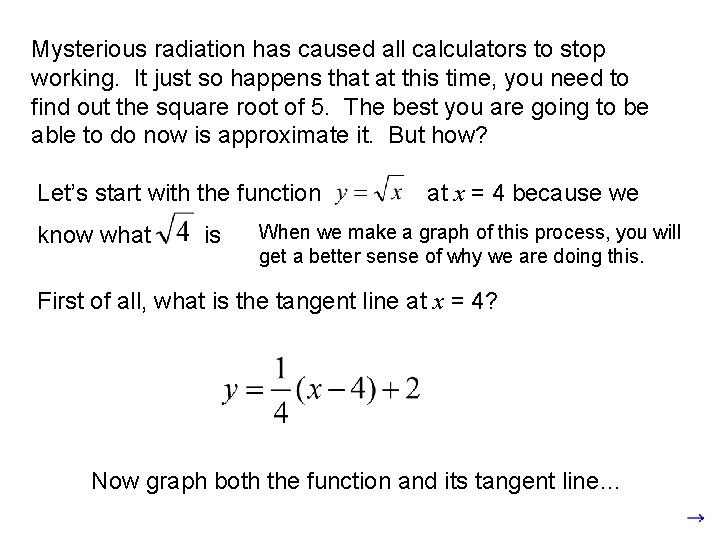
Mysterious radiation has caused all calculators to stop working. It just so happens that at this time, you need to find out the square root of 5. The best you are going to be able to do now is approximate it. But how? Let’s start with the function know what is at x = 4 because we When we make a graph of this process, you will get a better sense of why we are doing this. First of all, what is the tangent line at x = 4? Now graph both the function and its tangent line…

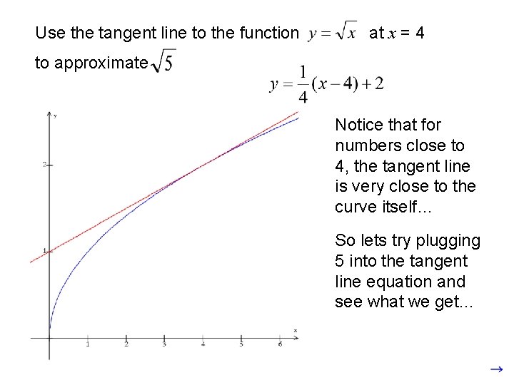
Use the tangent line to the function at x = 4 to approximate Notice that for numbers close to 4, the tangent line is very close to the curve itself… So lets try plugging 5 into the tangent line equation and see what we get…

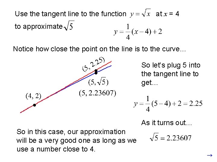
Use the tangent line to the function at x = 4 to approximate Notice how close the point on the line is to the curve… 5) 2. 2 So let’s plug 5 into (5, the tangent line to get… (4, 2) As it turns out… So in this case, our approximation will be a very good one as long as we use a number close to 4.

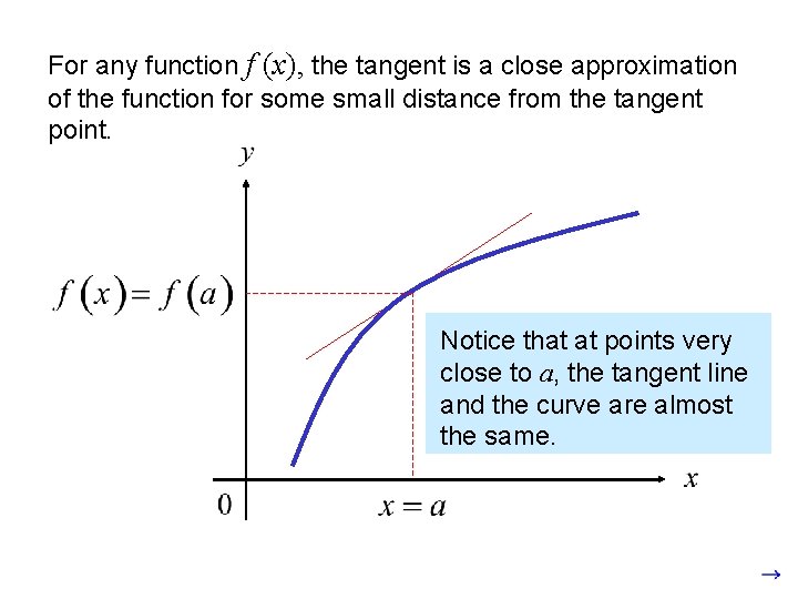
For any function f (x), the tangent is a close approximation of the function for some small distance from the tangent point. Notice that at points very close to a, the tangent line and the curve are almost the same.

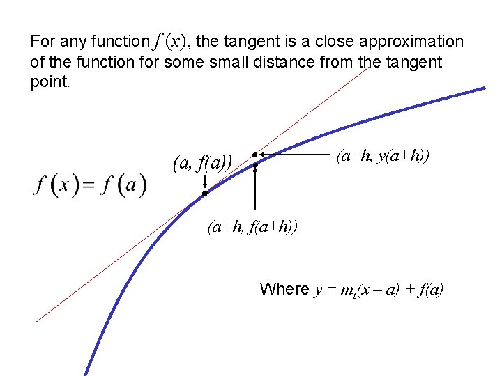
For any function f (x), the tangent is a close approximation of the function for some small distance from the tangent point. (a, f(a)) (a+h, y(a+h)) (a+h, f(a+h)) Where y = mt(x – a) + f(a)

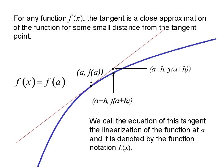
For any function f (x), the tangent is a close approximation of the function for some small distance from the tangent point. (a, f(a)) (a+h, y(a+h)) (a+h, f(a+h)) We call the equation of this tangent the linearization of the function at a and it is denoted by the function notation L(x).

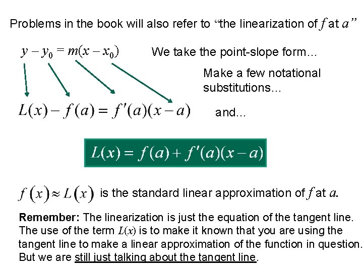
Problems in the book will also refer to “the linearization of f at a” y – y 0 = m(x – x 0) We take the point-slope form… Make a few notational substitutions… and… is the standard linear approximation of f at a. Remember: The linearization is just the equation of the tangent line. The use of the term L(x) is to make it known that you are using the tangent line to make a linear approximation of the function in question. But we are still just talking about the tangent line.

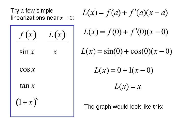
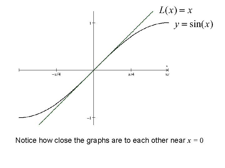
Try a few simple linearizations near x = 0: The graph would look like this:

Notice how close the graphs are to each other near x = 0

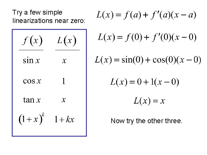
Try a few simple linearizations near zero: Now try the other three.

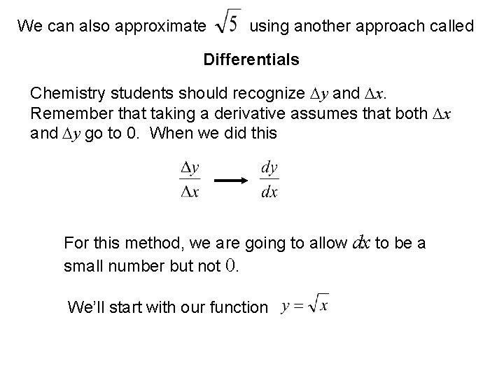
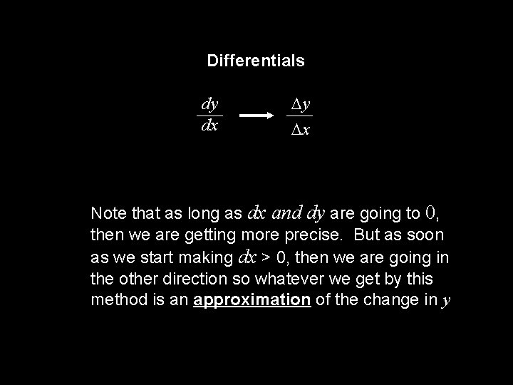
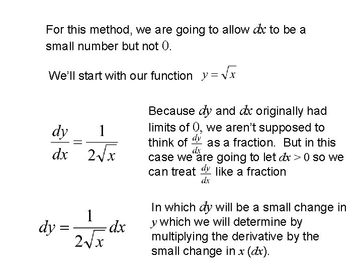
We can also approximate using another approach called Differentials Chemistry students should recognize y and x. Remember that taking a derivative assumes that both x and y go to 0. When we did this For this method, we are going to allow dx to be a small number but not 0. We’ll start with our function

Differentials dy dx y x Note that as long as dx and dy are going to 0, then we are getting more precise. But as soon as we start making dx > 0, then we are going in the other direction so whatever we get by this method is an approximation of the change in y

For this method, we are going to allow dx to be a small number but not 0. We’ll start with our function Because dy and dx originally had limits of 0, we aren’t supposed to think of as a fraction. But in this case we are going to let dx > 0 so we can treat like a fraction In which dy will be a small change in y which we will determine by multiplying the derivative by the small change in x (dx).

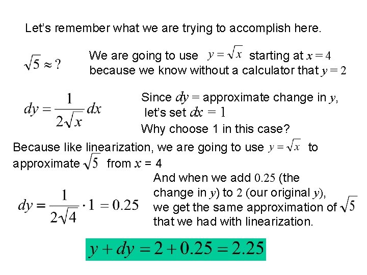
Let’s remember what we are trying to accomplish here. We are going to use starting at x = 4 because we know without a calculator that y = 2 Since dy = approximate change in y, let’s set dx = 1 Why choose 1 in this case? Because like linearization, we are going to use to approximate from x = 4 And when we add 0. 25 (the change in y) to 2 (our original y), we get the same approximation of that we had with linearization.

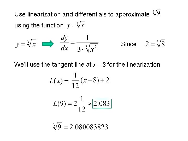
Use linearization and differentials to approximate using the function Since We’ll use the tangent line at x = 8 for the linearization

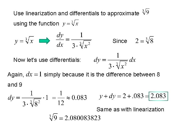
Use linearization and differentials to approximate using the function Since Now let’s use differentials: Again, simply because it is the difference between 8 and 9 Same as with linearization

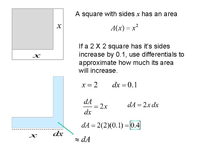
A square with sides x has an area If a 2 X 2 square has it’s sides increase by 0. 1, use differentials to approximate how much its area will increase.

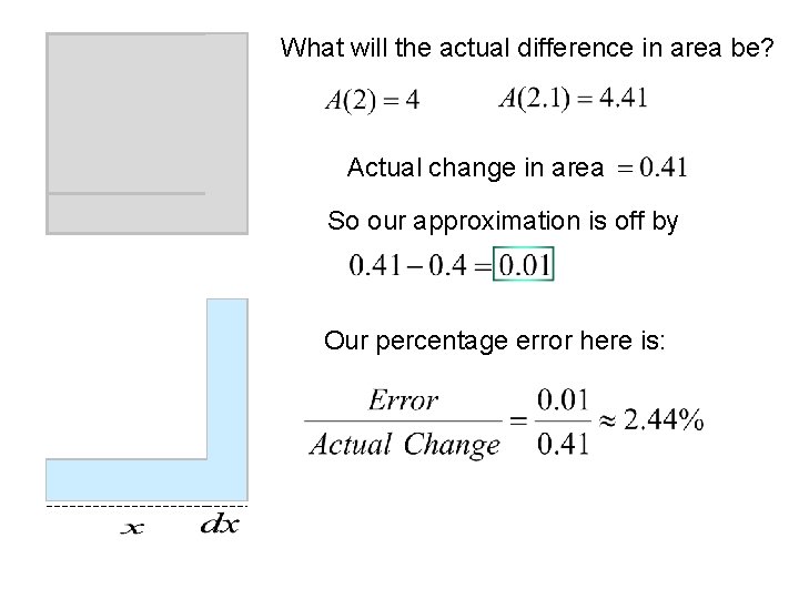
What will the actual difference in area be? Actual change in area So our approximation is off by Our percentage error here is: