4 5 Analyzing Lines of Best Fit Todays

4. 5 – Analyzing Lines of Best Fit Today’s learning goal is that students will be able to • Use residuals to determine how well lines of fit model data. • Distinguish between correlation and causation.

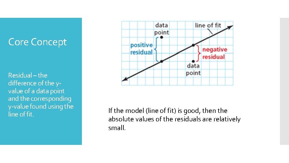
Core Concept Residual – the difference of the yvalue of a data point and the corresponding y-value found using the line of fit. If the model (line of fit) is good, then the absolute values of the residuals are relatively small.

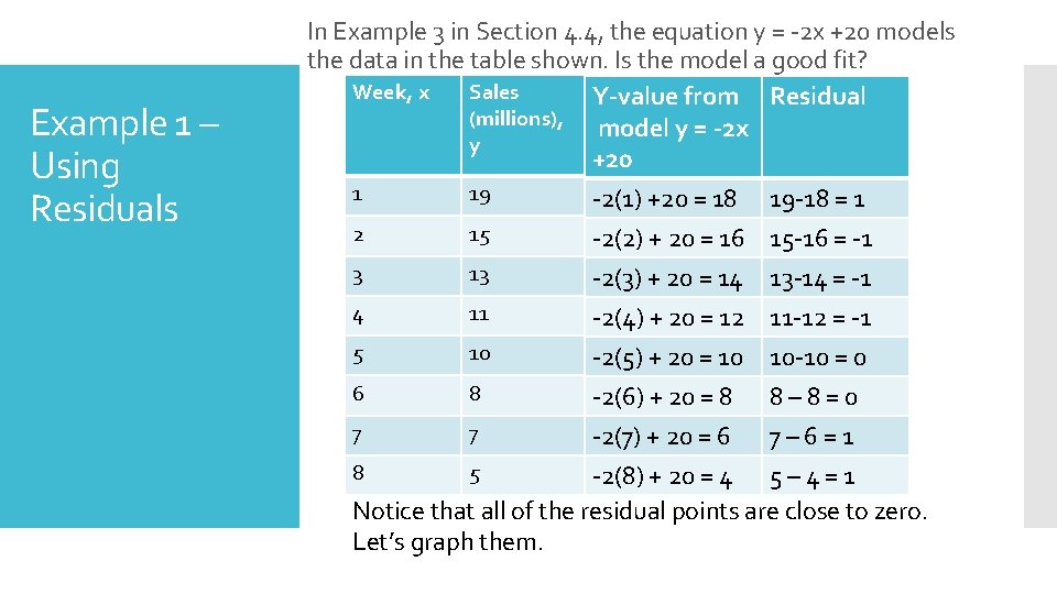
Example 1 – Using Residuals In Example 3 in Section 4. 4, the equation y = -2 x +20 models the data in the table shown. Is the model a good fit? Week, x Sales Y-value from Residual (millions), model y = -2 x y +20 1 19 -2(1) +20 = 18 19 -18 = 1 2 15 -2(2) + 20 = 16 15 -16 = -1 3 13 -2(3) + 20 = 14 13 -14 = -1 4 11 -2(4) + 20 = 12 11 -12 = -1 5 10 -2(5) + 20 = 10 10 -10 = 0 6 8 -2(6) + 20 = 8 8 – 8 = 0 7 7 -2(7) + 20 = 6 7 – 6 = 1 8 5 -2(8) + 20 = 4 5 – 4 = 1 Notice that all of the residual points are close to zero. Let’s graph them.

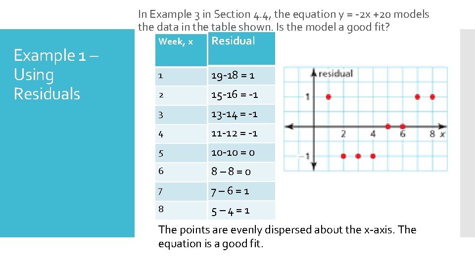
Example 1 – Using Residuals In Example 3 in Section 4. 4, the equation y = -2 x +20 models the data in the table shown. Is the model a good fit? Residual Week, x 1 19 -18 = 1 2 15 -16 = -1 3 13 -14 = -1 4 11 -12 = -1 5 10 -10 = 0 6 8– 8=0 7 7– 6=1 8 5– 4=1 The points are evenly dispersed about the x-axis. The equation is a good fit.

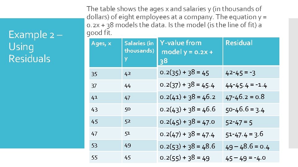
Example 2 – Using Residuals The table shows the ages x and salaries y (in thousands of dollars) of eight employees at a company. The equation y = 0. 2 x + 38 models the data. Is the model (is the line of fit) a good fit. Ages, x Salaries (in Y-value from Residual thousands) model y = 0. 2 x + y 38 0. 2(35) + 38 = 45 42 -45 = -3 35 42 37 44 0. 2(37) + 38 = 45. 4 44 -45. 4 = -1. 4 41 47 0. 2(41) + 38 = 46. 2 47 -46. 2 = 0. 8 43 50 0. 2(43) + 38 = 46. 6 50 -46. 6 = 3. 4 45 52 0. 2(45) + 38 = 47. 0 52 -47 = 5 47 51 0. 2(47) + 38 = 47. 4 51 -47. 4 = 3. 6 53 49 0. 2(53) + 38 = 48. 6 49 – 48. 6 = 0. 4 55 45 0. 2(55) + 38 = 49 45 – 49 = -4. 0

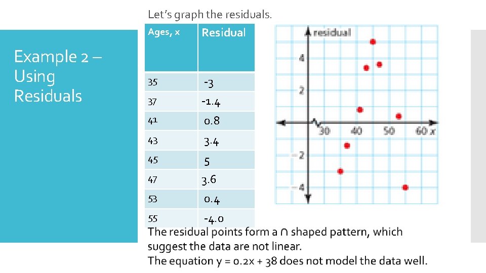
Let’s graph the residuals. Example 2 – Using Residuals Ages, x Residual 35 -3 37 -1. 4 41 0. 8 43 3. 4 45 5 47 3. 6 53 0. 4 55 -4. 0

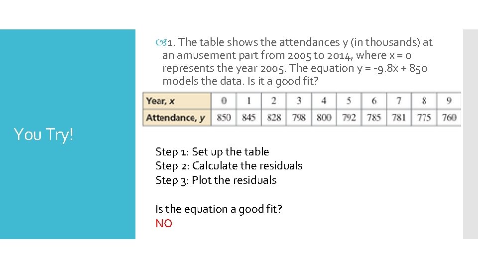
1. The table shows the attendances y (in thousands) at an amusement part from 2005 to 2014, where x = 0 represents the year 2005. The equation y = -9. 8 x + 850 models the data. Is it a good fit? You Try! Step 1: Set up the table Step 2: Calculate the residuals Step 3: Plot the residuals Is the equation a good fit? NO

Finding Lines of Best Fit Graphing calculators use a method called linear regression to find a precise line of fit called a line of best fit. A graphing calculator often gives a value r, called the correlation coefficient. Values of r range from -1 to 1. When r is close to -1, there is a strong negative correlation. When r is close to 1, there is a strong positive correlation. When r = 0, there is no correlation. When r is close to 0, the correlation is weak.

Correlation and Causation – when the change in one variable causes the change in another variable. When there is causation, there is a strong correlation. A strong correlation does not necessarily imply causation.

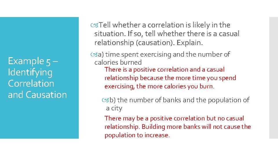
Tell whether a correlation is likely in the situation. If so, tell whethere is a casual relationship (causation). Explain. Example 5 – Identifying Correlation and Causation a) time spent exercising and the number of calories burned There is a positive correlation and a casual relationship because the more time you spend exercising, the more calories you burn. b) the number of banks and the population of a city There may be a positive correlation but no casual relationship. Building more banks will not cause the population to increase.

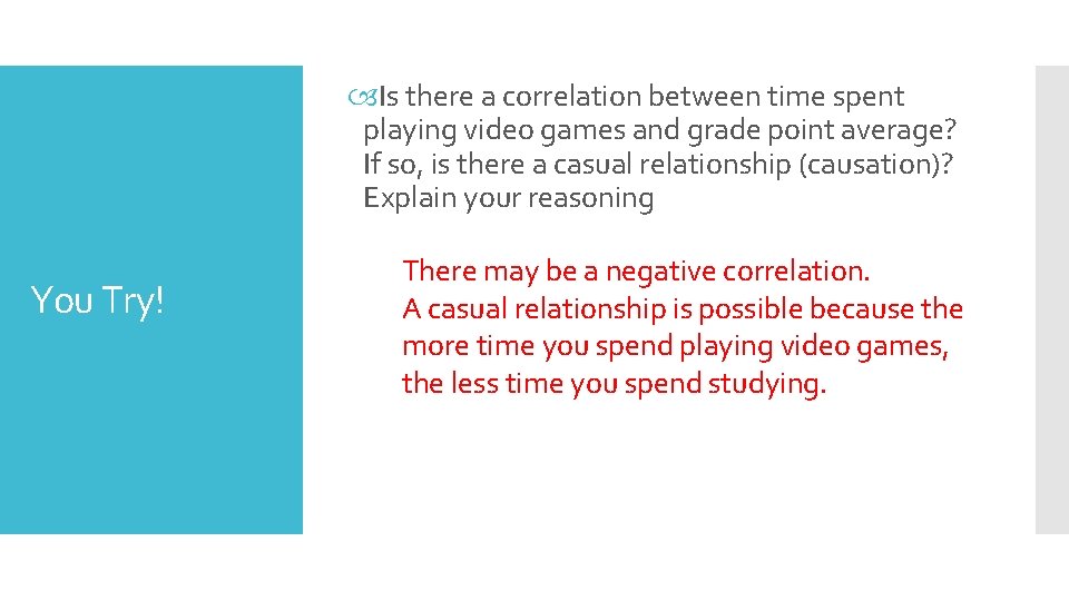
Is there a correlation between time spent playing video games and grade point average? If so, is there a casual relationship (causation)? Explain your reasoning You Try! There may be a negative correlation. A casual relationship is possible because the more time you spend playing video games, the less time you spend studying.