4 2 Polynomial Functions and Models Understand the

4. 2 Polynomial Functions and Models • Understand the graphs of polynomial functions • Evaluate and graph piecewise-defined functions • Use polynomial regression to model data Copyright © 2018, 2014, 2010 Pearson Education, Inc. All Rights Reserved

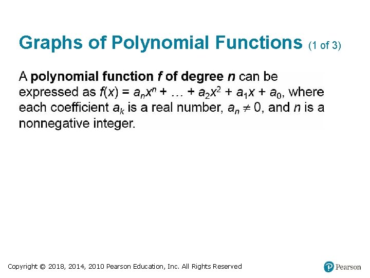
Graphs of Polynomial Functions (1 of 3) Copyright © 2018, 2014, 2010 Pearson Education, Inc. All Rights Reserved

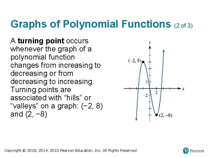
Graphs of Polynomial Functions (2 of 3) A turning point occurs whenever the graph of a polynomial function changes from increasing to decreasing or from decreasing to increasing. Turning points are associated with “hills” or “valleys” on a graph: (− 2, 8) and (2, − 8) Copyright © 2018, 2014, 2010 Pearson Education, Inc. All Rights Reserved

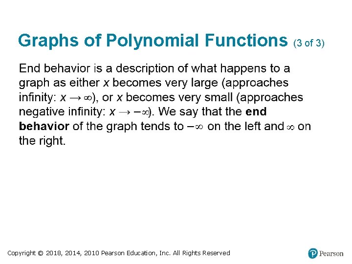
Graphs of Polynomial Functions (3 of 3) Copyright © 2018, 2014, 2010 Pearson Education, Inc. All Rights Reserved

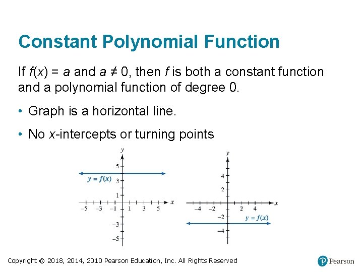
Constant Polynomial Function If f(x) = a and a ≠ 0, then f is both a constant function and a polynomial function of degree 0. • Graph is a horizontal line. • No x-intercepts or turning points Copyright © 2018, 2014, 2010 Pearson Education, Inc. All Rights Reserved

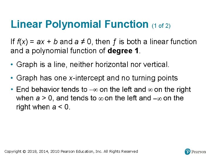
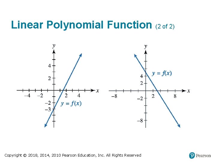
Linear Polynomial Function (1 of 2) If f(x) = ax + b and a ≠ 0, then ƒ is both a linear function and a polynomial function of degree 1. • Graph is a line, neither horizontal nor vertical. • Graph has one x-intercept and no turning points Copyright © 2018, 2014, 2010 Pearson Education, Inc. All Rights Reserved

Linear Polynomial Function (2 of 2) Copyright © 2018, 2014, 2010 Pearson Education, Inc. All Rights Reserved

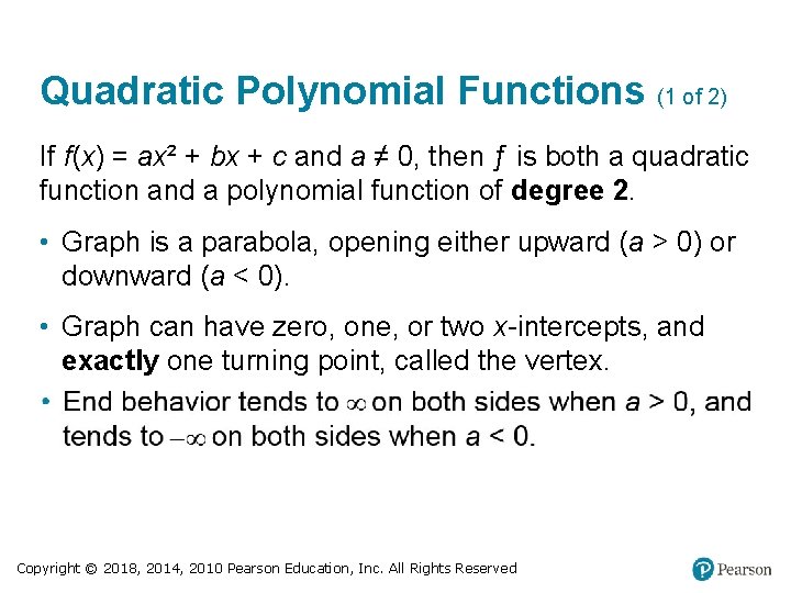
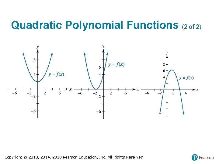
Quadratic Polynomial Functions (1 of 2) If f(x) = ax² + bx + c and a ≠ 0, then ƒ is both a quadratic function and a polynomial function of degree 2. • Graph is a parabola, opening either upward (a > 0) or downward (a < 0). • Graph can have zero, one, or two x-intercepts, and exactly one turning point, called the vertex. Copyright © 2018, 2014, 2010 Pearson Education, Inc. All Rights Reserved

Quadratic Polynomial Functions (2 of 2) Copyright © 2018, 2014, 2010 Pearson Education, Inc. All Rights Reserved

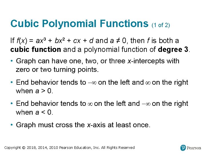
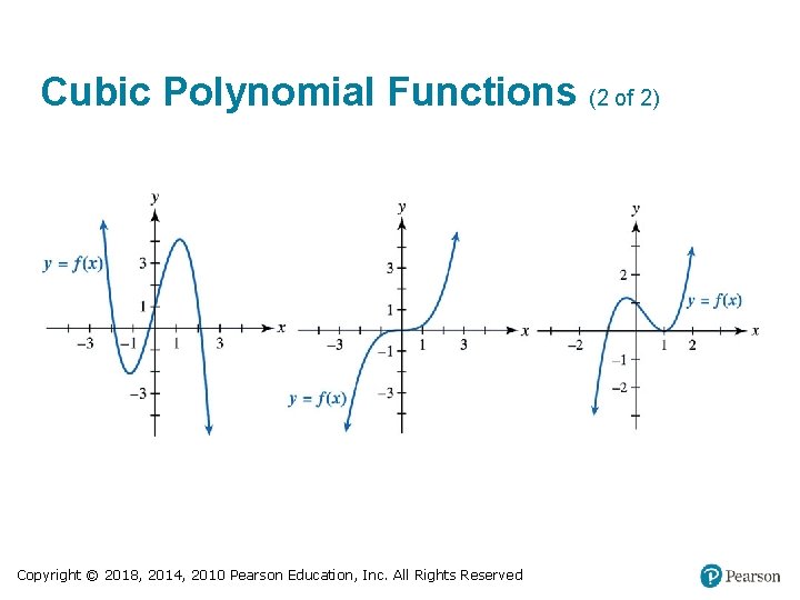
Cubic Polynomial Functions (1 of 2) If f(x) = ax³ + bx² + cx + d and a ≠ 0, then f is both a cubic function and a polynomial function of degree 3. Copyright © 2018, 2014, 2010 Pearson Education, Inc. All Rights Reserved

Cubic Polynomial Functions (2 of 2) Copyright © 2018, 2014, 2010 Pearson Education, Inc. All Rights Reserved

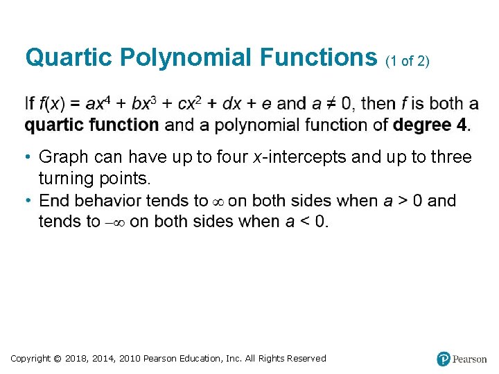
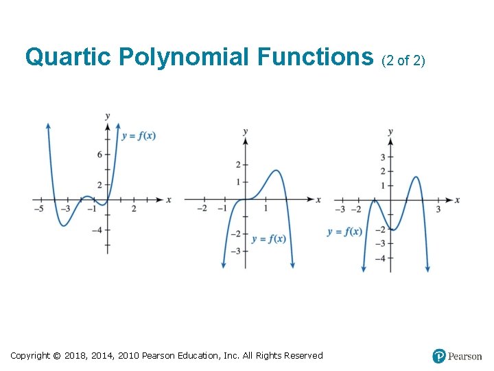
Quartic Polynomial Functions (1 of 2) • Graph can have up to four x-intercepts and up to three turning points. Copyright © 2018, 2014, 2010 Pearson Education, Inc. All Rights Reserved

Quartic Polynomial Functions (2 of 2) Copyright © 2018, 2014, 2010 Pearson Education, Inc. All Rights Reserved

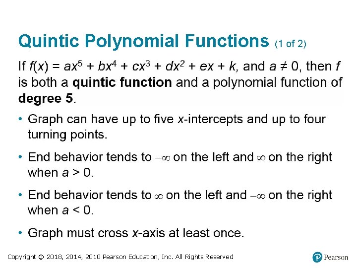
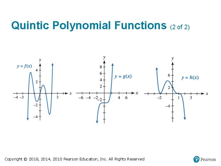
Quintic Polynomial Functions (1 of 2) Copyright © 2018, 2014, 2010 Pearson Education, Inc. All Rights Reserved

Quintic Polynomial Functions (2 of 2) Copyright © 2018, 2014, 2010 Pearson Education, Inc. All Rights Reserved

Degree, x-intercepts, and Turning Points The graph of a polynomial function of degree n, with n ≥ 1, has at most n x-intercepts and at most n − 1 turning points. Copyright © 2018, 2014, 2010 Pearson Education, Inc. All Rights Reserved

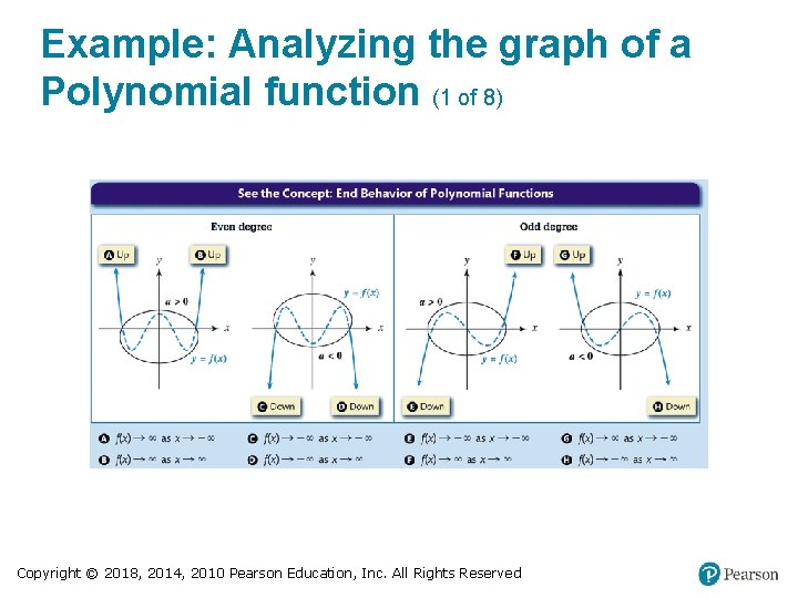
Example: Analyzing the graph of a Polynomial function (1 of 8) Copyright © 2018, 2014, 2010 Pearson Education, Inc. All Rights Reserved

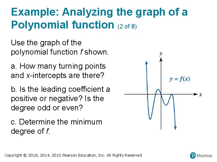
Example: Analyzing the graph of a Polynomial function (2 of 8) Use the graph of the polynomial function f shown. a. How many turning points and x-intercepts are there? b. Is the leading coefficient a positive or negative? Is the degree odd or even? c. Determine the minimum degree of f. Copyright © 2018, 2014, 2010 Pearson Education, Inc. All Rights Reserved

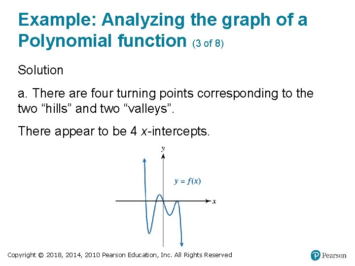
Example: Analyzing the graph of a Polynomial function (3 of 8) Solution a. There are four turning points corresponding to the two “hills” and two “valleys”. There appear to be 4 x-intercepts. Copyright © 2018, 2014, 2010 Pearson Education, Inc. All Rights Reserved

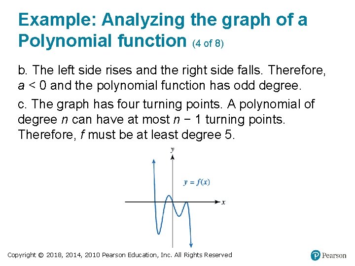
Example: Analyzing the graph of a Polynomial function (4 of 8) b. The left side rises and the right side falls. Therefore, a < 0 and the polynomial function has odd degree. c. The graph has four turning points. A polynomial of degree n can have at most n − 1 turning points. Therefore, f must be at least degree 5. Copyright © 2018, 2014, 2010 Pearson Education, Inc. All Rights Reserved

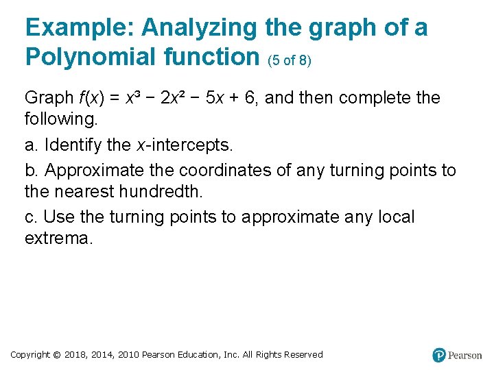
Example: Analyzing the graph of a Polynomial function (5 of 8) Graph f(x) = x³ − 2 x² − 5 x + 6, and then complete the following. a. Identify the x-intercepts. b. Approximate the coordinates of any turning points to the nearest hundredth. c. Use the turning points to approximate any local extrema. Copyright © 2018, 2014, 2010 Pearson Education, Inc. All Rights Reserved

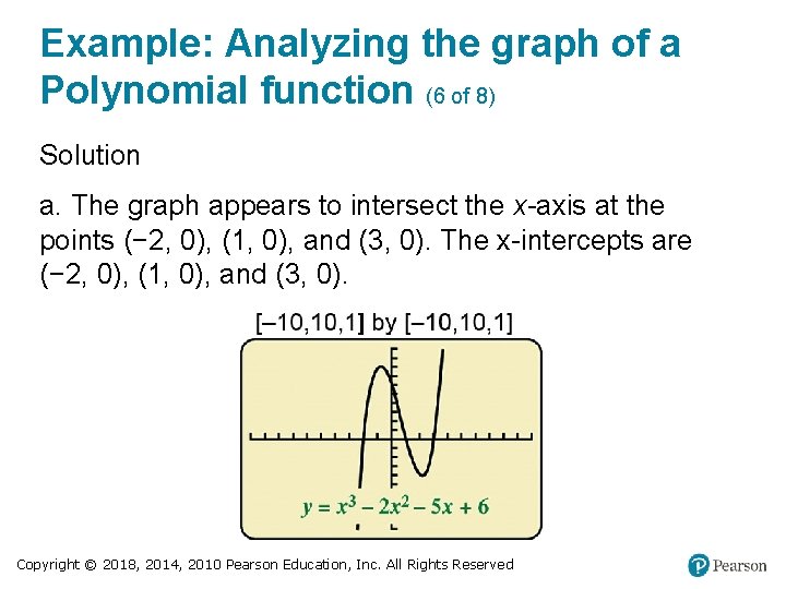
Example: Analyzing the graph of a Polynomial function (6 of 8) Solution a. The graph appears to intersect the x-axis at the points (− 2, 0), (1, 0), and (3, 0). The x-intercepts are (− 2, 0), (1, 0), and (3, 0). Copyright © 2018, 2014, 2010 Pearson Education, Inc. All Rights Reserved

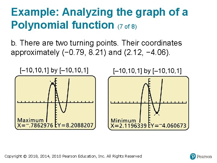
Example: Analyzing the graph of a Polynomial function (7 of 8) b. There are two turning points. Their coordinates approximately (− 0. 79, 8. 21) and (2. 12, − 4. 06). Copyright © 2018, 2014, 2010 Pearson Education, Inc. All Rights Reserved

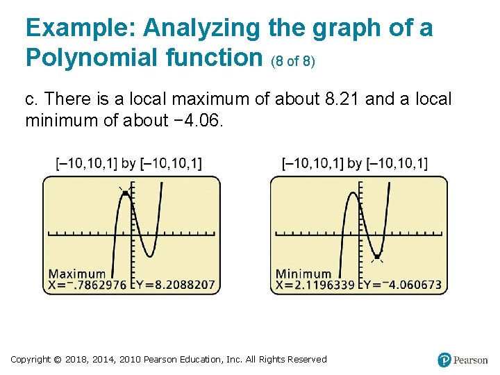
Example: Analyzing the graph of a Polynomial function (8 of 8) c. There is a local maximum of about 8. 21 and a local minimum of about − 4. 06. Copyright © 2018, 2014, 2010 Pearson Education, Inc. All Rights Reserved

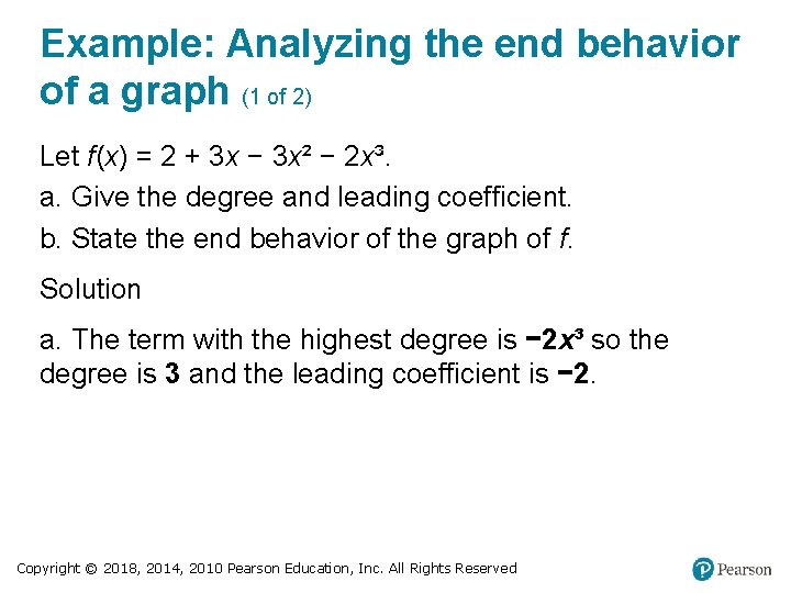
Example: Analyzing the end behavior of a graph (1 of 2) Let f(x) = 2 + 3 x − 3 x² − 2 x³. a. Give the degree and leading coefficient. b. State the end behavior of the graph of f. Solution a. The term with the highest degree is − 2 x³ so the degree is 3 and the leading coefficient is − 2. Copyright © 2018, 2014, 2010 Pearson Education, Inc. All Rights Reserved

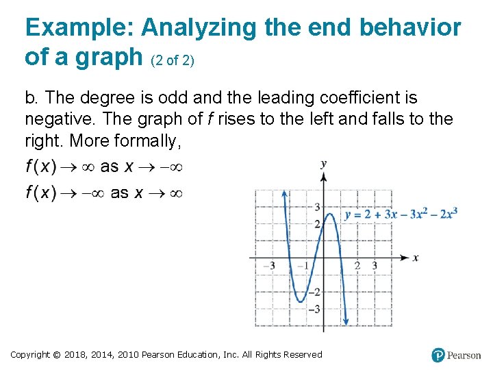
Example: Analyzing the end behavior of a graph (2 of 2) b. The degree is odd and the leading coefficient is negative. The graph of f rises to the left and falls to the right. More formally, Copyright © 2018, 2014, 2010 Pearson Education, Inc. All Rights Reserved

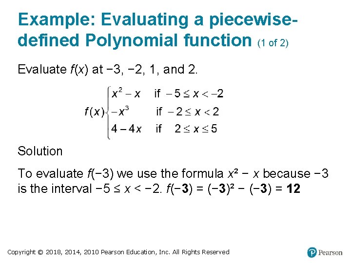
Example: Evaluating a piecewisedefined Polynomial function (1 of 2) Evaluate f(x) at − 3, − 2, 1, and 2. Solution To evaluate f(− 3) we use the formula x² − x because − 3 is the interval − 5 ≤ x < − 2. f(− 3) = (− 3)² − (− 3) = 12 Copyright © 2018, 2014, 2010 Pearson Education, Inc. All Rights Reserved

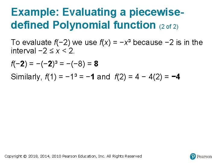
Example: Evaluating a piecewisedefined Polynomial function (2 of 2) To evaluate f(− 2) we use f(x) = −x³ because − 2 is in the interval − 2 ≤ x < 2. f(− 2) = −(− 2)³ = −(− 8) = 8 Similarly, f(1) = − 1³ = − 1 and f(2) = 4 − 4(2) = − 4 Copyright © 2018, 2014, 2010 Pearson Education, Inc. All Rights Reserved

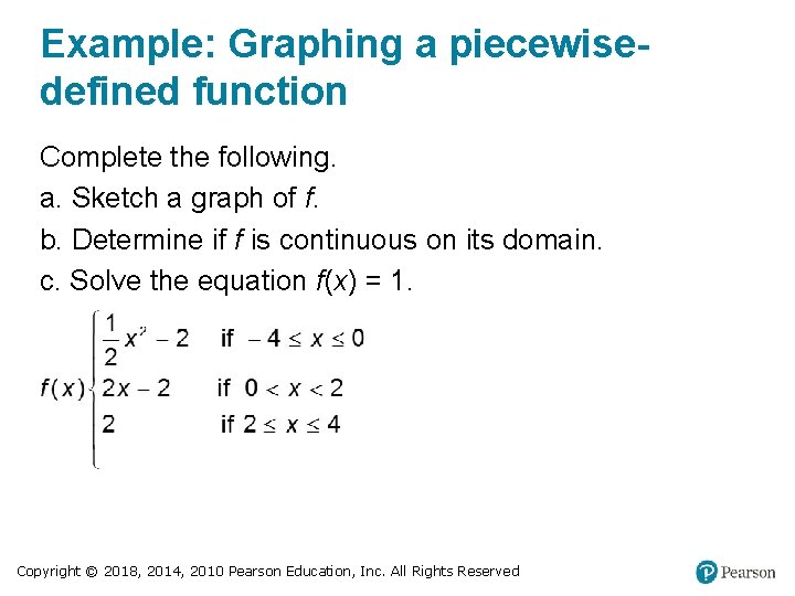
Example: Graphing a piecewisedefined function Complete the following. a. Sketch a graph of f. b. Determine if f is continuous on its domain. c. Solve the equation f(x) = 1. Copyright © 2018, 2014, 2010 Pearson Education, Inc. All Rights Reserved

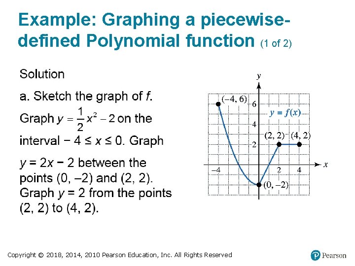
Example: Graphing a piecewisedefined Polynomial function (1 of 2) Copyright © 2018, 2014, 2010 Pearson Education, Inc. All Rights Reserved

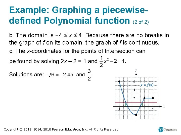
Example: Graphing a piecewisedefined Polynomial function (2 of 2) b. The domain is − 4 ≤ x ≤ 4. Because there are no breaks in the graph of f on its domain, the graph of f is continuous. Copyright © 2018, 2014, 2010 Pearson Education, Inc. All Rights Reserved

Polynomial Regression We now have the mathematical understanding to model the data presented in the introduction to this section: polynomial modeling. We can use least-squares regression, which was also discussed in previous sections, for linear and quadratic functions. Copyright © 2018, 2014, 2010 Pearson Education, Inc. All Rights Reserved

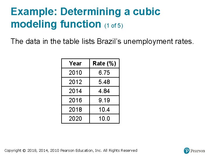
Example: Determining a cubic modeling function (1 of 5) The data in the table lists Brazil’s unemployment rates. Year Rate (%) 2010 6. 75 2012 5. 48 2014 4. 84 2016 9. 19 2018 10. 4 2020 10. 0 Copyright © 2018, 2014, 2010 Pearson Education, Inc. All Rights Reserved

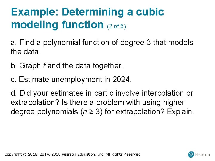
Example: Determining a cubic modeling function (2 of 5) a. Find a polynomial function of degree 3 that models the data. b. Graph f and the data together. c. Estimate unemployment in 2024. d. Did your estimates in part c involve interpolation or extrapolation? Is there a problem with using higher degree polynomials (n ≥ 3) for extrapolation? Explain. Copyright © 2018, 2014, 2010 Pearson Education, Inc. All Rights Reserved

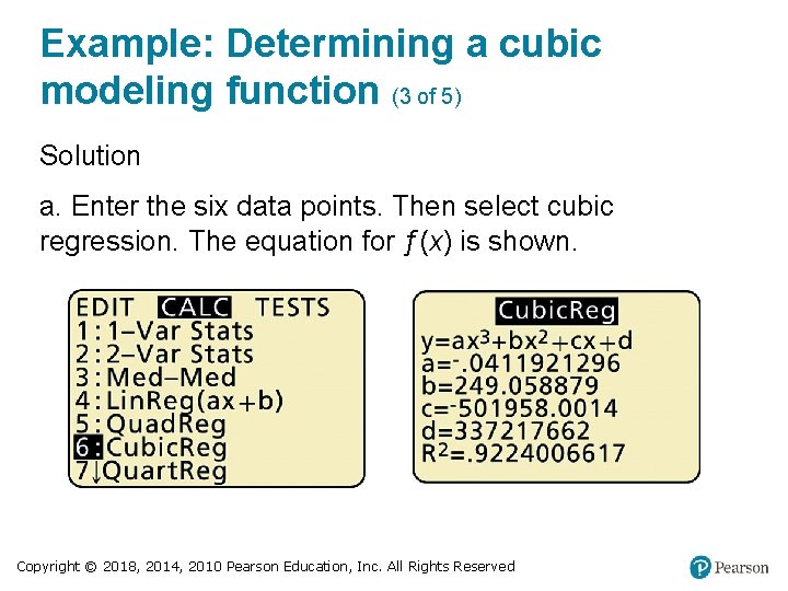
Example: Determining a cubic modeling function (3 of 5) Solution a. Enter the six data points. Then select cubic regression. The equation for ƒ(x) is shown. Copyright © 2018, 2014, 2010 Pearson Education, Inc. All Rights Reserved

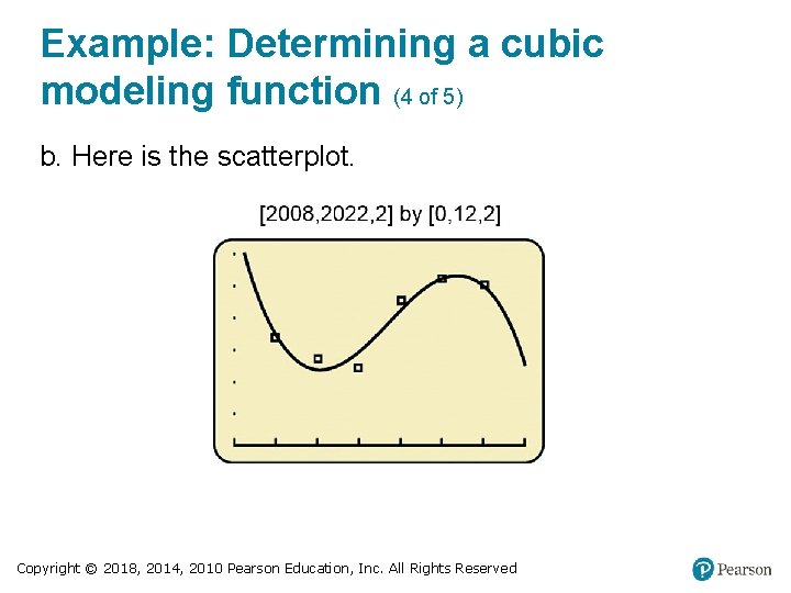
Example: Determining a cubic modeling function (4 of 5) b. Here is the scatterplot. Copyright © 2018, 2014, 2010 Pearson Education, Inc. All Rights Reserved

Example: Determining a cubic modeling function (5 of 5) c. f(2024) ≈ − 6. 58, which is incorrect because the employment rate cannot be negative. Copyright © 2018, 2014, 2010 Pearson Education, Inc. All Rights Reserved