4 0 ROOT LOCUS OBJECTIVE Determination of root

4. 0 ROOT LOCUS OBJECTIVE ~ Determination of root from the characteristic equation by using graphical solution. ~ Rules on sketching the root locus. ~ Analysis of closed-loop using root locus
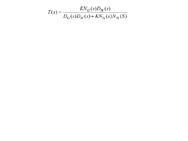
 H(s) = KG(S)H(s) =")
KG(S) H(s) = KG(S)H(s) =

Vector Representation of Complex Numbers • Any complex number, a vector. can be graphically represented by • The complex number can also be described in the form of magnitude M and angle θ , as. • If a complex number is substituted into a complex function, another complex number will result. Example, if
 + E(s) Y(s) KG(s) B(s) H(s) Open-loop transfer function")
Root locus concept Consider R(s) + E(s) Y(s) KG(s) B(s) H(s) Open-loop transfer function If and where and
=1 ~ Number and position of zeros for")
Closed-loop transfer function with unity feedback, H(s)=1 ~ Number and position of zeros for open-loop and closed-loop are the same ~ Position of poles for the closed-loop depend on the position of poles, zeros and K. Characteristic equation is If . Let and Its open-loop transfer function . and its closed-loop as ~ Position of poles for the closed-loop depend on the position of poles, zeros and K of the open-loop. transfer function.

As K varies the closed-loop poles follow similarly and form a locus. For that we define Root locus is a locus of charateristic equation as K varie from 0 to . Refering to a characteristic equation Let say Re-arrange -1 is a complex number where

Magnitude condition Re-arrange where and is the magnitude from a test point to open-loop poles is. the magnitude from a test point to open-loop zeros Since each complex factor can be thought of as a vector, the magnitude M, of F(s) at any point s, is
 at any point s, is")
Angle condition The angle, θ, of F(s) at any point s, is

m 1 x mm x x x s-plane s n 1 nn

satah s s O O
 at the")
Evaluation of a complex function via vectors • Given , find F(s) at the point. • Vector originating at the zero at -1 is • Vector originating at the pole at the origin is • Vector originating at the pole at -2 is
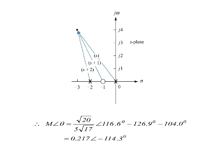

Evaluation of a complex function via vectors Solution:

Evaluation of a complex function via vectors Solution: 944 -66 -72 j -378 Answer:

Root Locus • Root Locus technique can be used to analyze and design the effect of loop gain upon the system’s transient response and stability.

Table 8. 1 Pole location as a function of gain for the system

Figure 8. 5 a. Pole plot from Table 8. 1; b. root locus The representation of the paths of the closed loop poles as the gain is varied is called root locus.

Root Locus • As gain K varies, for gain less than 25, the poles are real >>> overdamped • For K=25, the poles are real and multiple>>> critically damped • For K more than 25, the poles consist of real and imaginary parts >>> underdamped • For underdamped, the real part for the complex poles are always the same. • Settling Time is inversely proportional to the real part of the complex poles. Therefore, settling time remains the same under all condition of underdamped. • As K increase, the damping ratio diminishes, the percent of overshoot increases.

Figure 4. 17 Pole plot for an underdamped second-order system

Root Locus • The damped frequency of oscillation which is equal to the imaginary part of the pole also increase with an increase of gain, resulting in reduction of peak time. • Since the root locus never cross over to the right-half plane, the system is always stable.
 becomes")
Properties of root locus A pole, s, exists when the characteristic equation (denominator) becomes zero:

Referring to Table 8. 1, closed loop poles exist at -9. 47 and -0. 53 when the gain is 5. Substitute these values yields KG(s)H(s)= -1. The other points for Table 8. 1 show the same case.

Consider the point -2+j 3, if this point is a close-loop pole for some value of gain, then the angles of the zeros minus the angle of the poles must equal in odd multiple of 1800. Therefore, -2+j 3 is not the point on the root locus.

• Consider the point angle do add up to 180 o. • Replace the point as • the
 The number of branches of the")
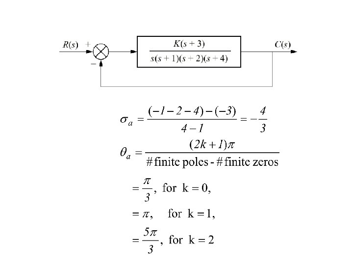
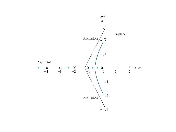
Sketching Root Locus Five rules to follow: 1) The number of branches of the roots locus equals the number of closed-loop poles. 2) The root locus is symmetrical about the real axis. 3) On the real axis, for K>0, the root locus exists to the left of an odd number of real axis, finite open loop poles and/or finite open loop zeros. 4) The root locus begins at the finite and infinite poles of G(s)H(s) and ends at the finite and infinite zeros of G(s)H(s). 5) The root locus approaches straight lines as asymptotes as the locus approaches infinity. The equation of the asymptotes is given by intercept and angle as follows: (the number of poles and zeros are equal if we include infinite and finite poles and zeros)

Sketching Root Locus • Rule 4

Sketching Root Locus
 Breakawayand Break-in points of locus from the real-axis Figure below shows a sketch")
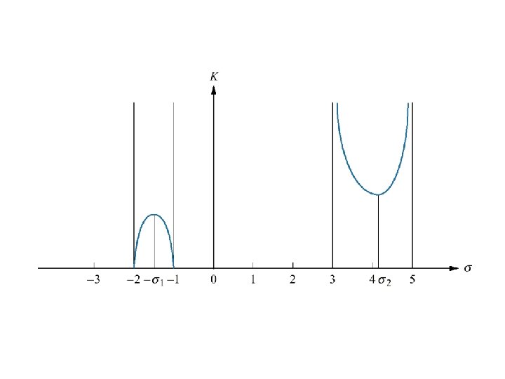
(6) Breakawayand Break-in points of locus from the real-axis Figure below shows a sketch using the first four rules: - 1 and 2 is called the breakaway and break-in point respectively.
 Breakawayand Break-in points of locus from the real-axis At the breakaway or break-in")
(6) Breakawayand Break-in points of locus from the real-axis At the breakaway or break-in point, the branches of the root locus form an angle 180 o/n with the real axis where n is the number of closedloop poles arriving and/or departing from the single breakaway or break-in on the real axis. As the two closed-loop poles at -1 and -2 at K=0 moving towards each other, the gain, K increases from a value of zero. Therefore, we conclude gain must be maximum between the open-loop poles at the breakaway point. The gain that increase above this value as the poles move into the complex plane. The gain will continue to increase to infinity as the close-loop poles move toward the open-loop zero. Therefore, we conclude that gain in the break-in point must be minimum gain found between the two zeros.
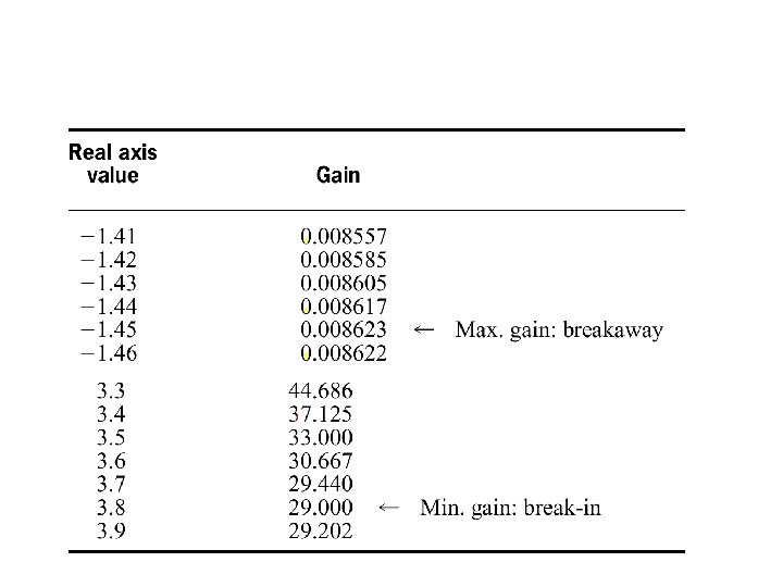

• Three methods to find the points at which the root locus break-in and breakaway: • First method: maximize and minimize the gain, K, using differential calculus. • Using the figure just now, = -1. 45 and 3. 82

• The second method: where zi and pi are the negative of the zero and pole values respectively of G(s)H(s). Repeat the example just now,
 Stability boundary of the locus We use the Routh-Hurwitz criteria determine the maximum")
(7) Stability boundary of the locus We use the Routh-Hurwitz criteria determine the maximum gain before instability and its frequency jω-axis point is a point on the root locus that separates the stable and unstable operation of a system. To find the jω-axis crossing with the rules: (1) forcing a row of zeros in the Routh table yield the gain (2) Going back one row to the even polynomial equation and solve the roots yield the frequency at the imaginary axis,

Only s 1 row can yield a row of zeros, thus

• Forming the even polynomial with K=9. 65, We conclude the system is stable for 0<= K<9. 65
 Angle of departure and arrival Finding angles of departure and arrival from the")
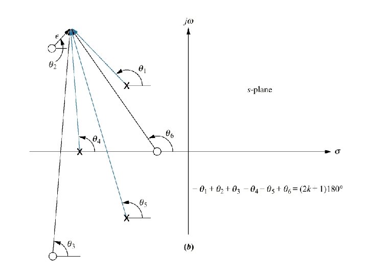
(8) Angle of departure and arrival Finding angles of departure and arrival from the complex poles and zeros.

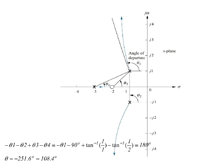
Find angle of departure from complex poles and sketch the root locus.

Locate point at Root Locus and Find Gain • • To find an exact coordinates of root locus as it crosses a radial line such as line for certain % of overshoot. Let say, we want to find root locus that crosses 0. 45 damping ratio line and the gain at that point.

Locate point at Root Locus and Find Gain • If a few test points along ζ =0. 45 line are selected, we can evaluate their angular sum and locate the point that angles add up to an odd multiple of 1800. Then, we can evaluate the gain at that point. • Example: the point at radius 2 (r=2) at the line, • Since the sum is not equal, the point is not on the root locus. • From the table, radius 0. 747 is on the root locus. Using the equation,

Transient Response Design • The effect of additional poles and zeros and the condition for justifying an approximation of a two-pole system is applied to close loop system and their root locus. • Conditions justifying a second order approximation are: (1) Higher order poles are much farther into the left of the s-plane than the dominant second-order pair of poles. (2) Closed-loop zeros near the closed-loop second-order pole pair are nearly cancelled by the close proximity of higher-order closed-loop poles. (3) Closed loop zeros not cancelled by the close proximity of higherorder closed-loop poles are far removed from the second order pole pair. Figure 8. 20(b) yields much better second order approximation than Figure 8. 20(a), since closed-loop pole is farther from the closed-loop second-order pair, p 1, and p 2. Figure 8. 20(d) yields much better second order approximation than Figure 8. 20(c), since closed-loop pole, p 3 is closer to cancelling closed-loop zero.

Figure 8. 20 Making second-order approximations

Third-order system gain design • Consider a system below, design the value of gain K to yield 1. 52% overshoot. Estimate the settling time, peak time, and steady-state error. Note that this is a third-order system with one zero. Root Locus is shown on Figure 8. 22

Figure 8. 22

• Breakaway points on the real axis can occur between 0 and -1 and between -1. 5 and -10, where the gain reaches a peak. • Using the root locus program, breakaway point is found at -0. 62 with a gain of 2. 511, and at 4. 4 with a gain of 28. 89. • Break-in point can occur between -1. 5 to -10, where the gain reaches a local minimum. Using the root locus program, break-in point is found at -2. 8 with gain 27. 91. • Assume system can be approximate by a second-order, underdamped system without any zeros. A 1. 52% overshoot correspond to a damping ratio of 0. 8. Sketch the damping ratio on the root locus. • Use root locus program to search along the 0. 8 damping ratio line for the point where angles add up to an odd multiple of 180 o. This is the point where root locus satisfy 1. 52%overshoot.

• Three points satisfy this criterion: -0. 87±j 0. 66, -1. 19±j 0. 90, and 4. 6±j 0. 3. 45, with a respective gains of 7. 36, 12. 79, 39. 64. • For each point, evaluate the settling time and peak time. • For steady state error, we get,

• Case 1 and Case 2 yield third closed-loop pole that are relatively far from the closedloop zero. For these two case, there are no pole-zero cancellation, therefore, a second order system approximation is not valid. • Case 3, third closed-loop pole that are relatively close to closed-loop zero. Therefore, a second order system approximation is valid.

Example: A plant of transfer function is feedback with a unity feedback. Sketch a root locus for Solution: Its characteristic equation is As the number of open-loop poles is 3, there will be 3 loci and the loci start at 0, -1 dan – 2. The locus on the real-axis

Satah-s -2 -1 As there is no zeros, the locus will end at asymtote lines, where This gives asymtote angles at , with real-axis crossing at

satah-s -2 -1 The loci will meet and depart at breakway point Rearrange Differentiate for the maximum value of K 60 o

Its root The probable root is – 0. 4 as it is on the locus The crossing at the boundary of stability 1 2 3 K K . and Range of gain for stability , replacing . The natural frequency is determined by taking to gives

Root Locus for positive feedback On the real axis, the root locus for positive-feedback system exists to the left of an even number of real-axis, finite open loop poles and/or finite open-loop zeros

Behavior at infinity: asymptotes:
- Slides: 58