4 0 Continuoustime Fourier Transform 4 1 From

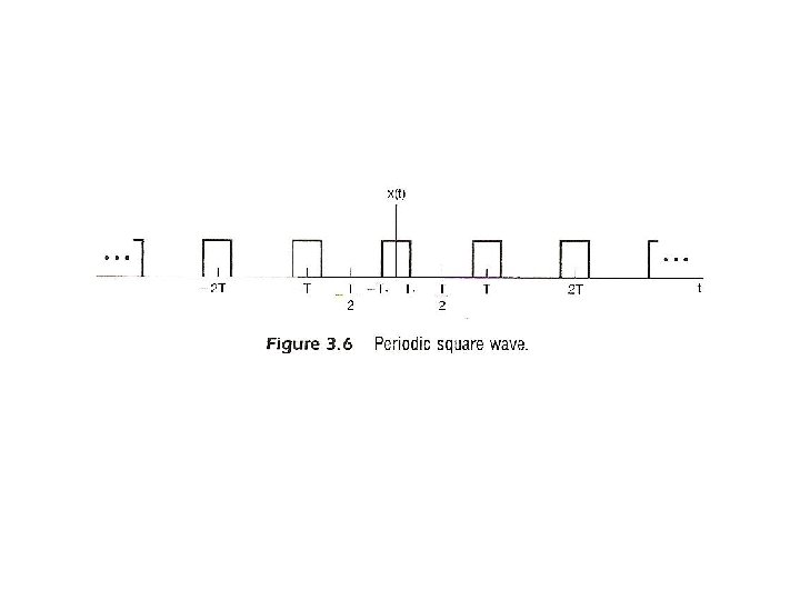
4. 0 Continuous-time Fourier Transform 4. 1 From Fourier Series to Fourier Transform l Fourier Series : for periodic signal See Fig. 3. 6, 3. 7, p. 193, 195, Fig, 4. 2, p. 286 of text – aperiodic : T , ω0 0

Harmonically Related Exponentials for Periodic Signals (P. 11 of 3. 0) T • All with period T: integer multiples of ω0 • Discrete in frequency domain

Fourier Transform T FS 0

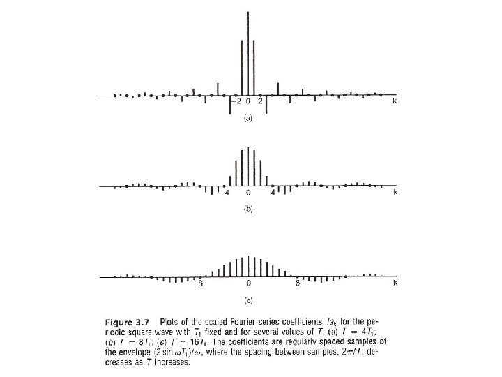
See Fig. 3. 6, 3. 7, p. 193, 195, Fig, 4. 2, p. 286 of text

l Considering – construct x(t), x(t)=0 for | t | > T 1

l Considering x(t), x(t)=0 for | t | > T 1 – Fourier series for – Defining envelope of Tak as X(jω)

l Considering – as x(t), x(t)=0 for | t | > T 1

spectrum, frequency domain Fourier Transform signal, time domain Inverse Fourier Transform pair, different expressions very similar format to Fourier Series for periodic signals

l Convergence – Given x(t) Issues

l Convergence Issues – It can be shown is obtainable (finite) for every ω zero energy for the difference signal differences at isolated points are possible converges to x(t) at continuous points, but to averages at discontinuities

l Convergence Issues – Dirichlet’s conditions (1) absolutely integrable (2) finite number of maxima and minima within any finite interval (3) finite number of discontinuities with finite values within any finite interval

Examples

Examples

l Fourier Transform for Periodic Signals – Unified Framework – Given x(t) (easy in one way)

Unified Framework: Fourier Transform for Periodic Signals T F S – If F

Examples • Example 4. 7, p. 298 of text

4. 2 Properties of Continuous-time Fourier Transform l Linearity

Linearity (P. 27 of 3. 0) l Linearity

l Time Shift linear phase shift (linear in frequency) with amplitude unchanged

Time Shift (P. 28 of 3. 0) phase shift linear in frequency with amplitude unchanged

Time Shift

Examples (P. 18 of 4. 0) • Example 4. 7, p. 298 of text

Sinusoidals

l Conjugation

l Conjugation (P. 32 of 3. 0) unique representation

Conjugation l Conjugation Unique representation for orthogonal bases

Even/Odd Properties l Conjugation Property − o X X X

Time Reversal Unique representation for orthogonal bases

l Time Reversal (P. 29 of 3. 0) the effect of sign change for x(t) and ak are identical unique representation for orthogonal basis

Even/Odd Properties x(t) both real and even − Time Reversal l l x(t) real and odd

l Differentiation/Integration dc term

l Differentiation (P. 33 of 3. 0)

Differentiation Enhancing higher frequencies De-emphasizing lower frequencies Deleting DC term ( =0 for ω=0)

Integration dc term Enhancing lower frequencies (accumulation effect) De-emphasizing higher frequencies Accumulation (smoothing effect) Undefined for ω=0

l Parseval’s Relation total energy: energy per unit time integrated over the time total energy: energy per unit frequency integrated over the frequency

l Time/Frequency Scaling (time reversal) See Fig. 4. 11, p. 296 of text

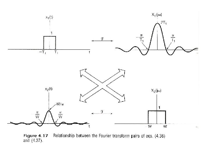
– inverse relationship between signal “width” in time/frequency domains

Single Frequency

l Time Scaling (P. 30 of 3. 0) positive real number periodic with period T/α and fundamental frequency αω0 ak unchanged, but x(αt) and each harmonic component are different

Data Transmission 1 1 0 1 T: bit duration pulse width : bit rate W : bandwidth

l Duality – time/frequency domains are kind of “symmetric” except for a sign change (and a factor of 2 ) --- “two domains” See Fig. 4. 17, p. 310 of text

Duality 0

(P. 10 of 4. 0) spectrum, frequency domain Fourier Transform signal, time domain Inverse Fourier Transform pair, different expressions very similar format to Fourier Series for periodic signals

Signal Representation in Two Domains Time Domain Basis Frequency Domain Basis

Signal Representation in Two Domains Time Domain Basis Frequency Domain Basis

Signal Representation in Two Domains Time Domain Basis Frequency Domain Basis

Signal Representation in Two Domains Time Domain Basis Frequency Domain Basis

Signal Representation in Two Domains Time Domain Basis Frequency Domain Basis (合成) (分析) (合成/分析)

l Duality – If any characteristics of signals in one domain implies some characteristics of signals in the other domain, the inverse is true except for a sign change (dual properties) modulation property

Modulation Property modulation: frequency translation shift in frequency Multiplication Property

l Convolution Property – System Input/Output Relationship superposition property closed-form solution frequency response

Input/Output Relationship (P. 5 of 3. 0) Time Domain l 0 0 Frequency Domain l

System Characterization l (P. 9 of 3. 0) Superposition Property – continuous-time – discrete-time – each frequency component never split to other frequency components, no convolution involved – desirable to decompose signals in terms of such eigenfunctions

Convolution Property Transfer Function Frequency Response

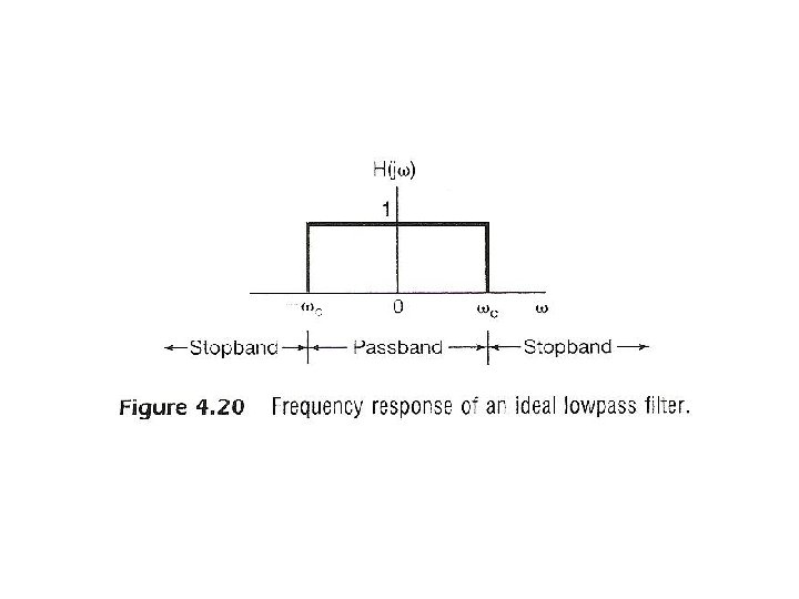
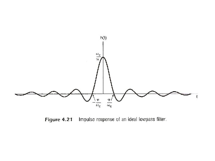
l Convolution Property – unit impulse response h(t) frequency response or transfer function H(jω) – convolution in time domain reduced to multiplication in frequency domain – cascade of two systems implies product of the two frequency responses, independent of the order of the cascade – example: filtering of signals See Fig. 4. 20, 4. 21, p. 318, 319 of text

Filtering of Signals 1 1 0 1 0

Realizable Lowpass Filter 0 0 0

l Differentiation/Integration (P. 33 of 4. 0) dc term

Integration 0 1 Duality 1 0

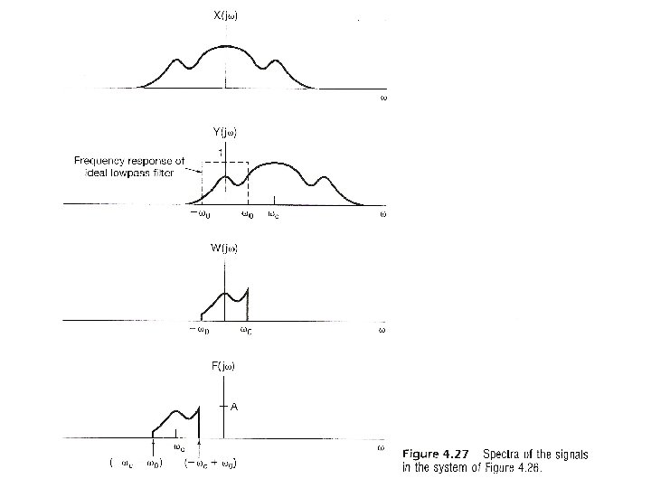
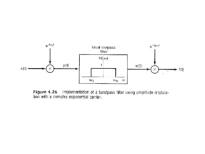
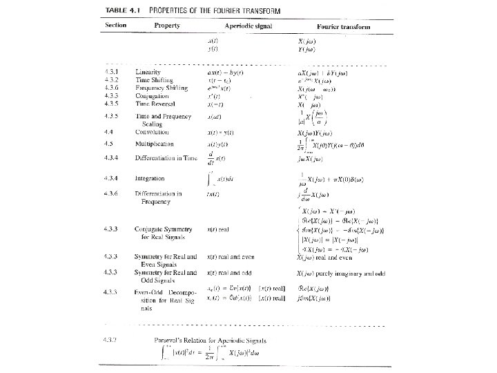
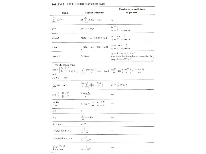
l Multiplication Property dual property of the convolution property – example: frequency-selective filtering with variable center frequency See Fig. 4. 26, 4. 27, p. 326 of text l Tables of Properties and Pairs See Tables. 4. 1, 4. 2, p. 328, 329 of text

Modulation Property (P. 53 of 4. 0) modulation: frequency translation shift in frequency Multiplication Property

Frequency Division Multiplexing

l Another Application Example systems described by differential equations: – closed-form solution

l Vector Space Interpretation of Fourier Transform – generalized Parseval’s Relation {X(jω) defined on -∞ < ω < ∞}=V: a vector space inner-product of two vectors(signals) can be evaluated in either the time domain or the frequency domain Parseval’s relation is a special case here: the magnitude (norm) of a vector can be evaluated in either the time domain or the frequency domain

l Vector Space Interpretation of Fourier Transform – considering the basis signal set

l Vector Space Interpretation of Fourier Transform – considering the basis signal set similar to the vector space of continuous-time signals – orthogonal bases but normalized, while makes sense considering operational definition

Examples • Example 4. 8, p. 299 of text

Examples • Example 4. 13, p. 310 of text – From Example 4. 2 by duality

Examples • Example 4. 19, p. 320 of text

Problem 4. 12, p. 336 of text

Problem 4. 13, p. 336 of text

Problem 4. 33, p. 345 of text

Problem 4. 35, p. 346 of text

Problem 4. 51, p. 354 of text, part (c) • An echo system x(t) y(t) α T h(t) …… x(t) y(t) T (-α) g(t)