383 11 C Linear Convolution We know that

383 11 -C 計算 Linear Convolution We know that when then (N points) (M points) (P points) But how do we implement it correctly? How do we choose P ? Note: When then FFTP: the P-point FFT ((a))P: a 除以 P 的餘數 IFFTP: the P-point inverse FFT

384 When then (Proof) Suppose that Here we apply ((a))P : the remainder of a after divided by P

[Discrete Circular Convolution and Discrete Linear Convolution] A discrete linear time-invariant (LTI) system can always be expressed a discrete linear convolution: However, the convolution implemented by the DFT is the discrete circular convolution: If then ((a))P : the remainder of a after divided by P 385

linear convolution: 386 circular convolution: For example, The condition where the circular convolution is equal to the linear convolution: (i) (iii)

387 The condition where the circular convolution is equal to the linear convolution: (i) (iii) (Proof): (Since P+n+1 -M P+1 -M N)

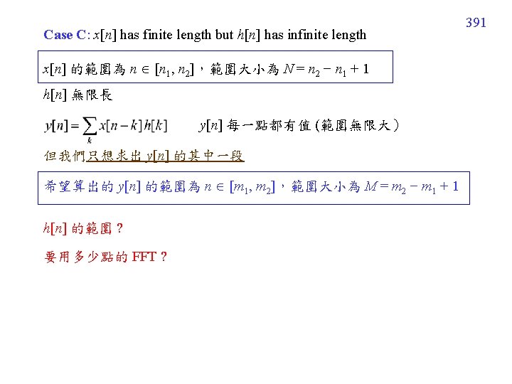
388 Linear Convolution 有幾種 Cases Case A: Both x[n] and h[n] have infinite lengths. (impossible) Case B: Both x[n] and h[n] have finite lengths. Case C: x[n] has infinite length but h[n] has finite length. Case D: x[n] has finite length but h[n] has infinite length. We focus on Case B. Case C and Case D can also be computed.

389 Case B: Both x[n] and h[n] have finite lengths. x[n] 的範圍為 n [n 1, n 2]，大小為 N = n 2 − n 1 + 1 h[n] 的範圍為 n [k 1, k 2]，大小為 K = k 2 − k 1 + 1 (n 1, k 1 can be nonzero) y[n] 的範圍? n 1 n 2 N y[n] h[n] x[n] n k 1 k 2 M n n 1+k 1 n 2+k 2 n N+M-1 Convolution output 的範圍以及 點數， 是學信號處理的人必需了解的常識

390 FFT implementation for Case B for n = 0, 1, 2, … , N− 1 for n = N, N+1 , … , P− 1 P N+M− 1 for n = 0, 1, 2, … , M− 1 for n = M, M+1 , … , P− 1 for n = n 1+k 1 , n 1+k 1+1, n 1+k 1+2, ……. , k 2 + n 2 i. e. , 取 output 的前面 N+M 1 個點

11 -D Relations between the Signal Length and the Convolution Algorithm 395 Suppose that x[n]: input, h[n]: the impulse response of the filter length(x[n]) = N, length(h[n]) = M (Both of them have finite lengths) We want to compute N M , y[n] = x[n] h[n]. The above convolution needs the P-point DFT, P M + N 1. complexity: O(P log 2 P)

396 [Case 1]: When M is a very small integer: Directly computing Number of multiplications for directly computing: N M Number of real multiplications for directly computing: 3 N M When using Number of real multiplications MULP: the number of multiplications for the P-point DFT When 3 N M , it is proper to do directly computing instead of applying the DFT.

397 Example: N = 126, M = 3, (difference, edge detection) (3/2)log 2 N = 10. 4659 When compute the number of real multiplications explicitly, using direct implementation: using the 128 -point DFT: using the 144 -point DFT: 3 N M = 1134,

398 Although in usual “directly computing” is not a good idea for convolution implementation, in the cases where (a) M is small (b) The filter has some symmetric relation using the directly computing method may be efficient for convolution implementation. Example: edge detection h[n] = [-0. 1, - 0. 3, -0. 6, 0, 0. 6, 0. 3, 0. 1] for n = -3 ~ 3

399 Example: smooth filter h[n] = [0. 1, 0. 2, 0. 4, 0. 2, 0. 1] for n = -2 ~ 2

400 [Case 2]: When M is not a very small integer but much less than N (N >> M): It is proper to divide the input x[n] into several parts: Each part has the size of L (L > M). x[n] (n = 0, 1, …. , N 1) x 1[n], x 2[n], x 3[n], ……. . , x. S[n] S = N/L , x[n] x 1[n] Section 1 means rounding toward infinite x 3[n] x. S-1[n] x 1[n] = x[n] for n = 0, 1, 2, …. , L 1, x 2[n] Section 2 x 2[n] = x[n + L] : Section s xs[n] = x[n + (s-1)L] for n = 0, 1, 2, …. , L 1, s = 1, 2, 3, …. , S x. S[n]

401 length = L length = M It should perform the P-point FFTs 2 S+1 times or 2 S times P L+M 1 Why?

402 Detail of Implementation Suppose that the P-point DFT is applied for each section when n < 0 and n N (1) First, determine L = P M + 1 (2) for n = 0, 1, 2, …. , L 1, for n = L, L+1, …. , N 1 for n = 0, 1, 2, …. , M 1, for n = M, M+1, …. , N 1 (3) Then calculate (4) Then, apply “overlapped addition” s = 1, 2, 3, …. , S S = N/L

403 運算量： 2 S MULP + 3 S P S N/L, P L+M 1 MULP: the number of multiplications for the P-point DFT 運算量： 2 S [(3 P/2)log 2 P] + 3 S P (理論值) S N/L, P L+M 1 (linear with N) 何時為 optimal? In practice, a computer program is applied to determine the optimal L.

optimal L (section length) 404 M (filter length)

405 注意： (1) Optimal section length is independent to N (2) If M is a fixed constant, then the complexity is linear with N, i. e. , O(N) 比較：使用原本方法時， complexity = O((N+M-1)log 2 (N+M-1)) (3) 實際上，需要考量 P-point FFT 的乘法量必需不多 P = L+M 1 例如，根據 page 403 的方法，算出當 M = 10 時， L = 41. 5439 為 optimal 但實際上，應該選 L = 39，因為此時 P = L+M 1 = 48 點的 DFT 有較少的 乘法量

406 [Case 3]: When M has the same order as N [Case 4]: When M is much larger than N [Case 5]: When N is a very small integer

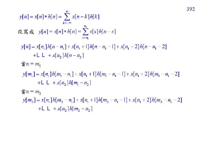
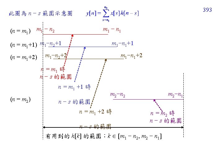
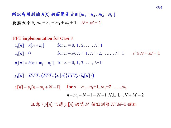
407 Sectioned Convolution for the Condition where One Sequence is Finite and the Other One is Infinite x[n] 0 for n 1 n n 2, length of x[n] = N = n 2 n 1 + 1, length of h[n] is infinite, and we want to calculate y[m] for m 1 m m 2, M = m 2 m 1 + 1. Suppose that M << N. In this case, we can try to partition x[n] into several sections. section 1: x 1[n] = x[n] for n = n 1 ~ n 1 + L 1, x 1[n] = 0 otherwise, section 2: x 2[n] = x[n] for n = n 1+ L ~ n 1 + 2 L 1, x 2[n] = 0 otherwise, section q: xq[n] = x[n] for n = n 1+ (q 1)L ~ n 1 + q. L 1, xq[n] = 0 otherwise,

Then we perform the convolution of xq[n] * h[n] for each of the sections by the method on pages 392 -394. (Since the length of xq[n] is L, it requires the P-point DFT, P L+M 1. Its complexity and the optimal section length can also be determined by the formulas on page 403. 408

11 -E Recursive Method for Convolution Implementation u[n]: unit step function Only two multiplications required for calculating each output. 409

410 h[n] = 0. 25 0. 6|n|

12. Fast Algorithm 的補充 12 -A Discrete Fourier Transform for Real Inputs DFT: 當 f [n] 為 real 時， F [m] = F*[N − m] *: conjugation 411

412 若我們要對兩個 real sequences f 1[n] ，f 2[n] 做 DFTs Step 1: f 3[n] = f 1[n] + j f 2[n] Step 2: F 3[m] = DFT{f 3[n]} Step 3: 只需一個 DFT 證明：由於 DFT 是一個 linear operation 又 F 1 [m] = F 1*[N − m] F 2 [m] = F 2*[N − m]

413 同理，當兩個 inputs 為 (1) pure imaginary (2) one is real and another one is pure imaginary 時，也可以用同樣的方法將運算量減半

• 若 input sequence 為 even f[n] = f[N-n]， 則 DFT output 也為 even F[n] = F[N-n] • 若 input sequence 為 odd f[n] = -f[N-n]， 則 DFT output 也為 odd F[n] = -F[N-n] 若 input sequence 為 odd and real， 則乘法量可減為 1/4 414

415 [Corollary 1] If it is known that the IDFTs of F 1[m] and F 2[m] are real, then the IDFTs of F 1[m] and F 2[m] can be implemented using only one IDFT: (Step 1) F 3[m] = F 1[m] + j F 2[m] (Step 2) f 3[n] = IDFT{F 3[m]} (Step 3) f 1[n] = Re {f 3[n]}, f 2[n] = Im{f 2[n]}, [Corollary 2] When x[n] and h[n] are both real, the computation loading of the convolution (or the sectioned convolution) of x[n] and h[n] can be halved.

12 -B Converting into Convolution 416 一般的 linear operation: (習慣上，把 k[m, n] 稱作 “kernel”) n = 0, 1, …. , N 1, m = 0, 1, …. , M 1 可以用矩陣 (matrix) 來表示 運算量為 MN 若為 linear time-invariant operation: k[m, n] = h[m n] (dependent on m, n 之間的差) n = 0, 1, …. , N 1, m = 0, 1, …. , M 1 m n 的範圍： 從 1 N 到 M 1， 全長 M + N 1 運算量為 Llog 2 L, L M+2 N 2

大致上，變成 convolution 後 總是可以節省運算量 例子A 可以改寫為 convolution 運算量為 M+N + Llog 2 L 例子B Linear Canonical Transform 417

418 General rules： 當k[m, n] 可以拆解成 A[m] B[m−n] C[n] 或 即可以使用 convolution

419 12 -C LUT (lookup table) 道理和背九九乘法表一樣 記憶體容量夠大時可用的方法 Problem: memory requirement wasting energy 九九乘法表的例子

421 (7) Key Factor (8) Imagination (9) 純粹意外

(1) Combination A (existing) 422 例： B (existing) 蒸汽機 車 火車 C (innovation) (2) Analog 例： A (existing) C (existing) B (existing) D (innovation) continuous Fourier transform continuous cosine transform discrete Fourier transform discrete cosine transform

423 (3) Connection A (existing) 例： 古典物 理學 C (innovation) 相對論 B (existing) 未能解釋的 光學現象 (4) Generalization A (existing) 保留某 些特性 將其他特性 推廣化 B (innovation) 例： Walsh transform 保留不需 乘法 將 1 推廣為 2 k Jacket transform

424 (5) Simplification 例： A (existing) 保留某 些特性 去除複雜 化的因素 DFT 保留 orthogonal, 正負號變化 B (innovation) 去除 無理數乘法 Walsh transform (6) Reverse A (existing) D (innovation) 電 B (existing) C (existing) 電生磁 磁生電 (法拉第定律) (安培定律) 磁