32931 Technology Research Methods Autumn 2017 Quantitative Research

32931 Technology Research Methods Autumn 2017 Quantitative Research Component Topic 4: Bivariate Analysis (Contingency Analysis and Regression Analysis) Lecturer: Mahrita Harahap Mahrita. Harahap@uts. edu. au B Math. Fin (Hons) M Stat (UNSW) Ph. D (UTS) mahritaharahap. wordpress. com/ teaching-areas Faculty of Engineering and Information Technology UTS CRICOS PROVIDER CODE: 00099 F

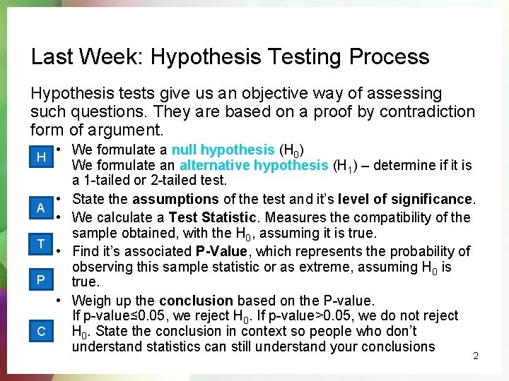
Last Week: Hypothesis Testing Process Hypothesis tests give us an objective way of assessing such questions. They are based on a proof by contradiction form of argument. H A T P C • We formulate a null hypothesis (H 0) We formulate an alternative hypothesis (H 1) – determine if it is a 1 -tailed or 2 -tailed test. • State the assumptions of the test and it’s level of significance. • We calculate a Test Statistic. Measures the compatibility of the sample obtained, with the H 0, assuming it is true. • Find it’s associated P-Value, which represents the probability of observing this sample statistic or as extreme, assuming H 0 is true. • Weigh up the conclusion based on the P-value. If p-value≤ 0. 05, we reject H 0. If p-value>0. 05, we do not reject H 0. State the conclusion in context so people who don’t understand statistics can still understand your conclusions 2

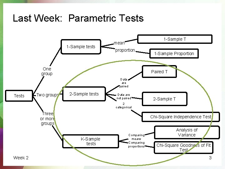
Last Week: Parametric Tests 1 -Sample tests 1 -Sample T mean proportion One group 1 -Sample Proportion Paired T Data are paired Tests Two groups 2 -Sample tests Data are not paired 2 -Sample T 2 categorical Three or more groups Chi-Square Independence Test K-Sample tests Week 2 Comparing means Comparing proportions Analysis of Variance Chi-Square Goodness of Fit Test 3

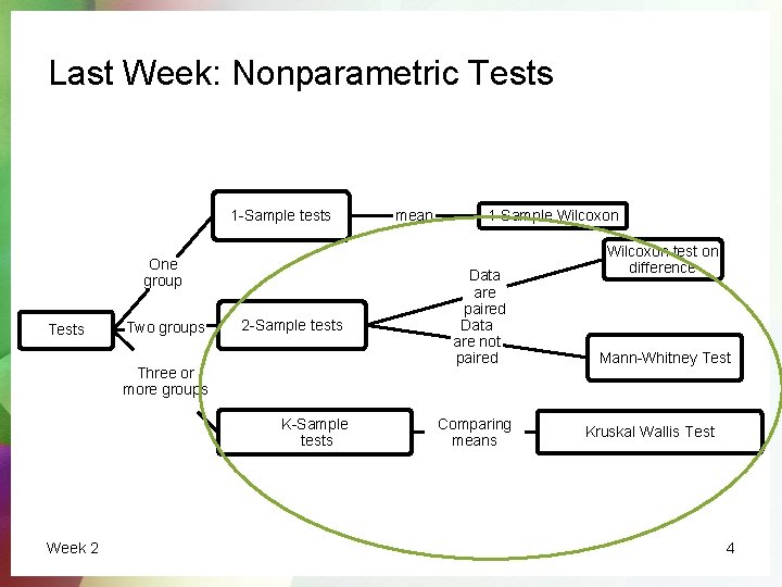
Last Week: Nonparametric Tests 1 -Sample tests One group Tests Two groups 2 -Sample tests Three or more groups K-Sample tests Week 2 mean 1 -Sample Wilcoxon Data are paired Data are not paired Comparing means Wilcoxon test on difference Mann-Whitney Test Kruskal Wallis Test 4

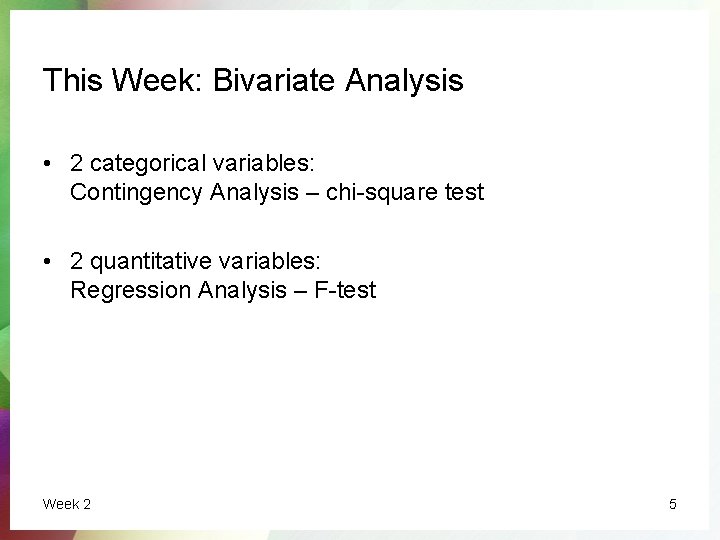
This Week: Bivariate Analysis • 2 categorical variables: Contingency Analysis – chi-square test • 2 quantitative variables: Regression Analysis – F-test Week 2 5

Contingency Analysis: Chi-Squared Test CATEGORICAL X CATEGORICAL Week 4 6

Chi-Squared Test In some situations, it is useful to look at the number of observations in each level of a categorical variable, or in each combination of two or more categorical variables This allows us to find relationships between two or more categorical variables. We can construct a contingency table (otherwise known as a two-way table or a crosstab) that contains this information. Week 4 7

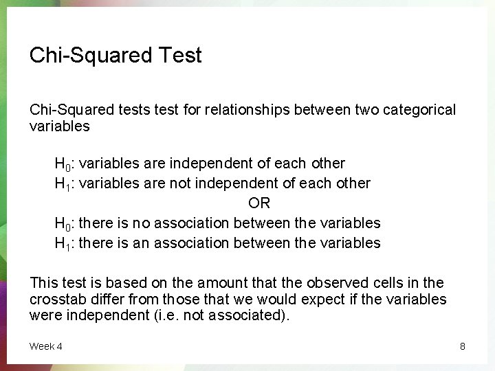
Chi-Squared Test Chi-Squared tests test for relationships between two categorical variables H 0: variables are independent of each other H 1: variables are not independent of each other OR H 0: there is no association between the variables H 1: there is an association between the variables This test is based on the amount that the observed cells in the crosstab differ from those that we would expect if the variables were independent (i. e. not associated). Week 4 8

Chi-Squared Test In order to test hypotheses on contingency tables, we need a table to test against. This table should reflect the case where there is no relationship between the variables. • Since we wish to ‘prove’ a relationship between the variables, if one exists. • Then H 0 will be that there is no relationship between the variables (i. e. independent or not associated) Week 4 9

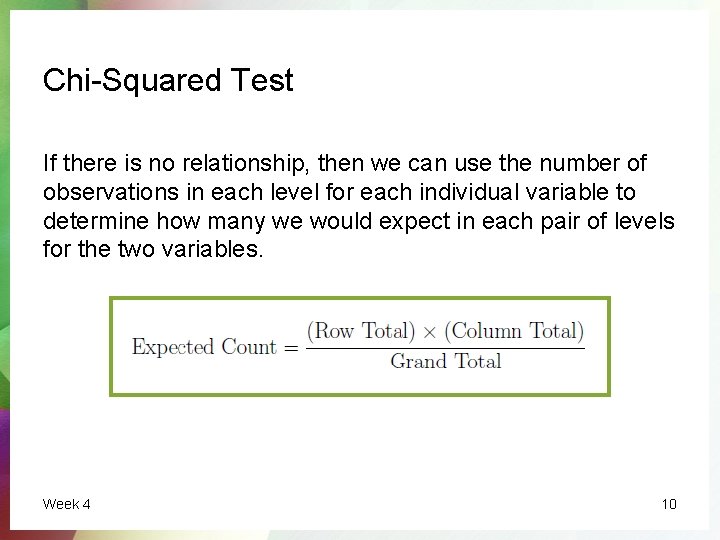
Chi-Squared Test If there is no relationship, then we can use the number of observations in each level for each individual variable to determine how many we would expect in each pair of levels for the two variables. Week 4 10

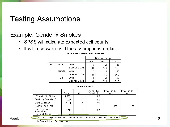
Chi-Squared Test: Assumptions We require there to be an adequate sample in each cell. As a rule of thumb, we need to have no more than 20% of the cells in the table with an expected cell count of less than 5 and no cells with an expected cell count of less than 1. If we do not have an adequate sample, then the test statistic (and hence the p-value) will be very sensitive to small changes in the sample counts. If this assumption is not valid, the equivalent nonparametric alternative test is called the Fisher’s Exact Test. 11

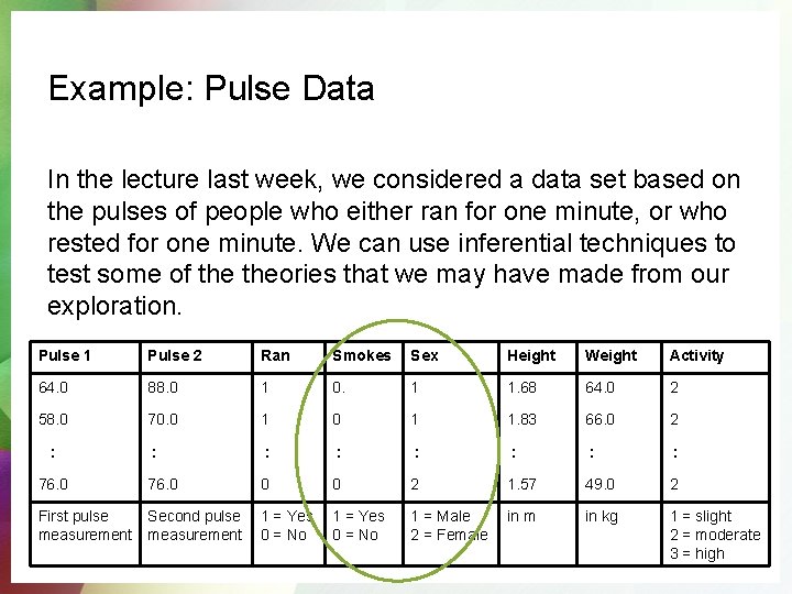
Example: Pulse Data In the lecture last week, we considered a data set based on the pulses of people who either ran for one minute, or who rested for one minute. We can use inferential techniques to test some of theories that we may have made from our exploration. Pulse 1 Pulse 2 Ran Smokes Sex Height Weight Activity 64. 0 88. 0 1 0. 1 1. 68 64. 0 2 58. 0 70. 0 1 1. 83 66. 0 2 : : 76. 0 0 0 2 1. 57 49. 0 2 First pulse measurement Second pulse measurement 1 = Yes 0 = No 1 = Male 2 = Female in m in kg 1 = slight 2 = moderate 3 = high :

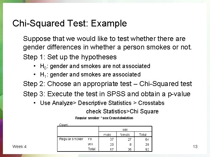
Chi-Squared Test: Example Suppose that we would like to test whethere are gender differences in whether a person smokes or not. Step 1: Set up the hypotheses • H 0: gender and smokes are not associated • H 1: gender and smokes are associated Step 2: Choose an appropriate test – Chi-Squared test Step 3: Execute the test in SPSS and obtain a p-value • Use Analyze> Descriptive Statistics > Crosstabs check Statistics>Chi Square Week 4 13

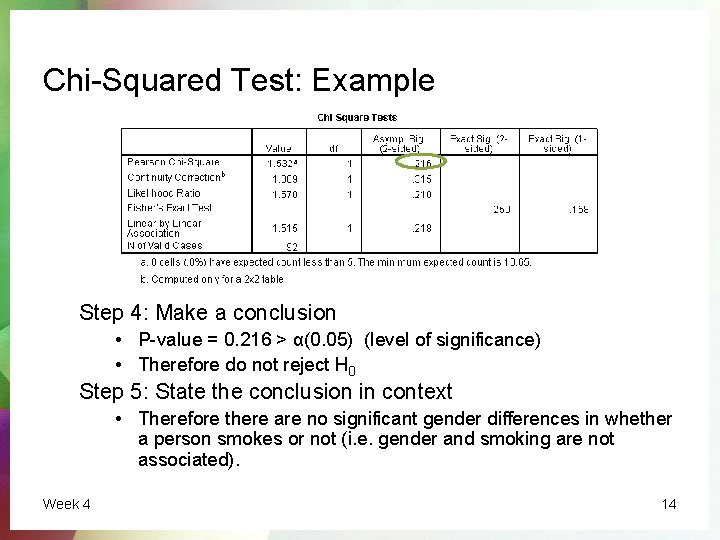
Chi-Squared Test: Example Step 4: Make a conclusion • P-value = 0. 216 > α(0. 05) (level of significance) • Therefore do not reject H 0 Step 5: State the conclusion in context • Therefore there are no significant gender differences in whether a person smokes or not (i. e. gender and smoking are not associated). Week 4 14

Testing Assumptions Example: Gender x Smokes • SPSS will calculate expected cell counts. • It will also warn us if the assumptions do fail. Week 4 15

Regression Analysis QUANTITATIVE X QUANTITATIVE Week 4 16

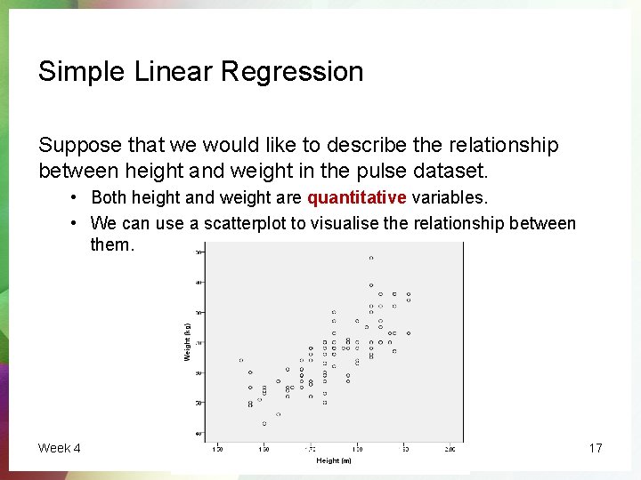
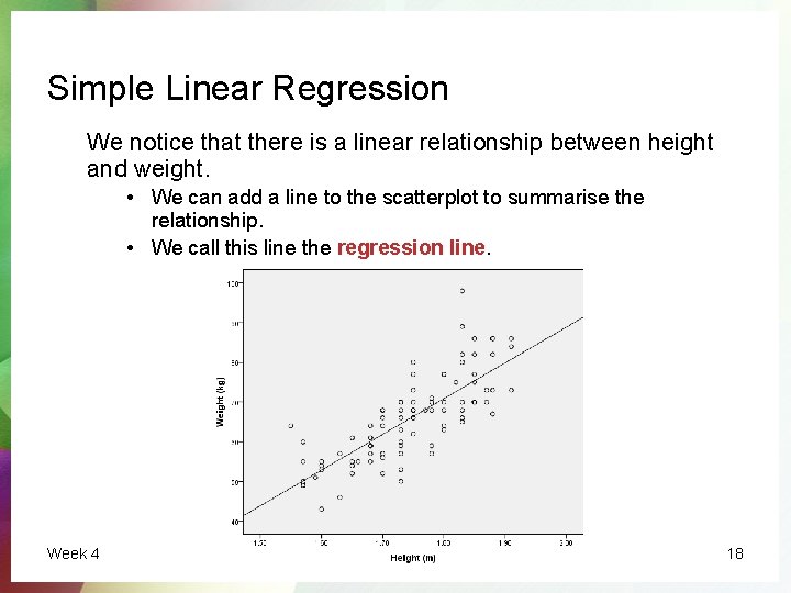
Simple Linear Regression Suppose that we would like to describe the relationship between height and weight in the pulse dataset. • Both height and weight are quantitative variables. • We can use a scatterplot to visualise the relationship between them. Week 4 17

Simple Linear Regression We notice that there is a linear relationship between height and weight. • We can add a line to the scatterplot to summarise the relationship. • We call this line the regression line. Week 4 18

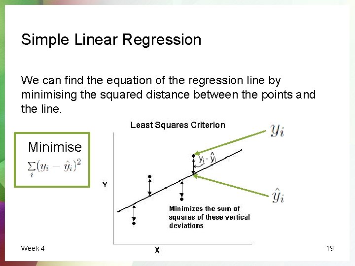
Simple Linear Regression We can find the equation of the regression line by minimising the squared distance between the points and the line. Minimise Week 4 19

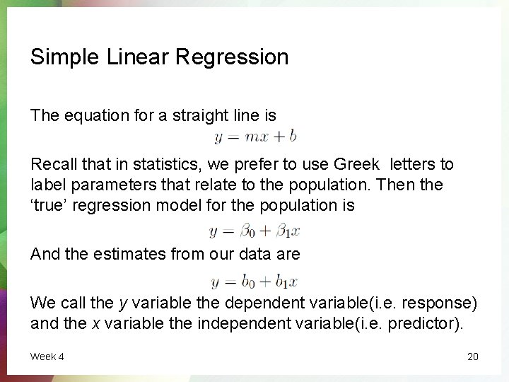
Simple Linear Regression The equation for a straight line is Recall that in statistics, we prefer to use Greek letters to label parameters that relate to the population. Then the ‘true’ regression model for the population is And the estimates from our data are We call the y variable the dependent variable(i. e. response) and the x variable the independent variable(i. e. predictor). Week 4 20

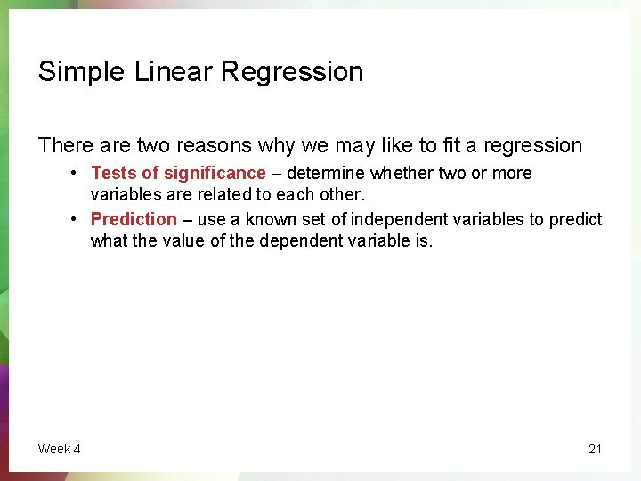
Simple Linear Regression There are two reasons why we may like to fit a regression • Tests of significance – determine whether two or more variables are related to each other. • Prediction – use a known set of independent variables to predict what the value of the dependent variable is. Week 4 21

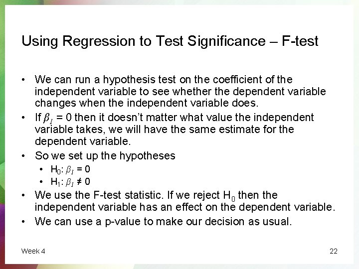
Using Regression to Test Significance – F-test • We can run a hypothesis test on the coefficient of the independent variable to see whether the dependent variable changes when the independent variable does. • If β 1 = 0 then it doesn’t matter what value the independent variable takes, we will have the same estimate for the dependent variable. • So we set up the hypotheses • H 0 : β 1 = 0 • H 1 : β 1 ≠ 0 • We use the F-test statistic. If we reject H 0 then the independent variable has an effect on the dependent variable. • We can use a p-value to make our decision as usual. Week 4 22

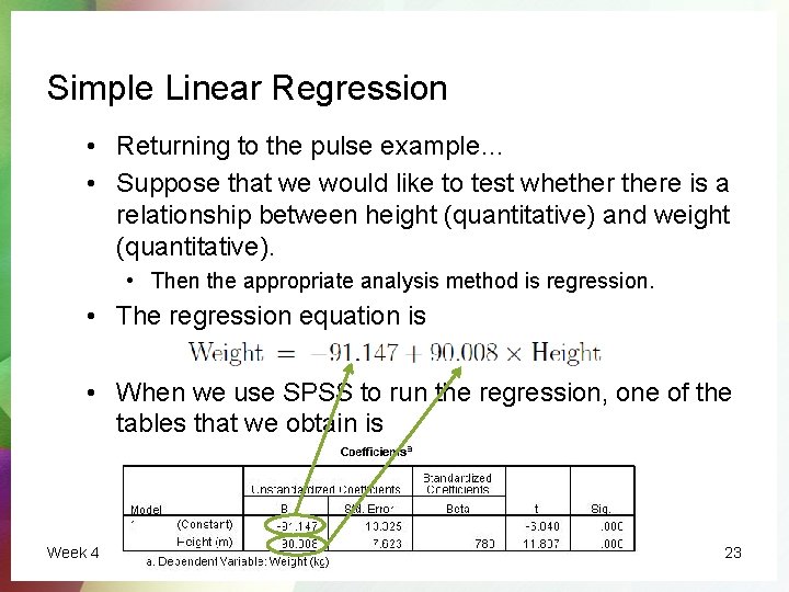
Simple Linear Regression • Returning to the pulse example… • Suppose that we would like to test whethere is a relationship between height (quantitative) and weight (quantitative). • Then the appropriate analysis method is regression. • The regression equation is • When we use SPSS to run the regression, one of the tables that we obtain is Week 4 23

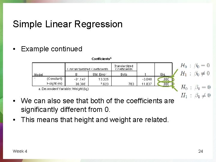
Simple Linear Regression • Example continued • We can also see that both of the coefficients are significantly different from 0. • This means that height and weight are related. Week 4 24

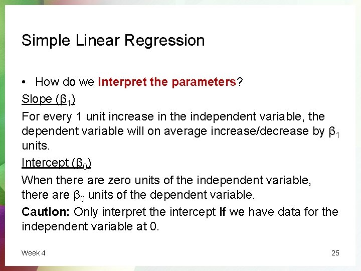
Simple Linear Regression • How do we interpret the parameters? Slope (β 1) For every 1 unit increase in the independent variable, the dependent variable will on average increase/decrease by β 1 units. Intercept (β 0) When there are zero units of the independent variable, there are β 0 units of the dependent variable. Caution: Only interpret the intercept if we have data for the independent variable at 0. Week 4 25

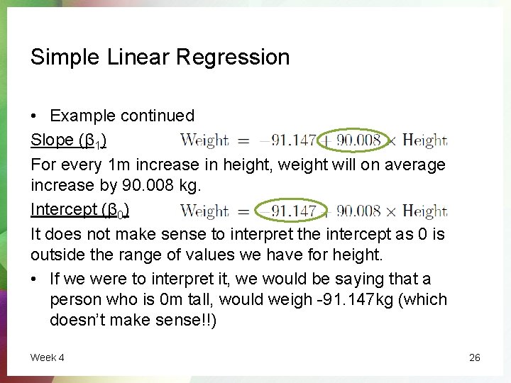
Simple Linear Regression • Example continued Slope (β 1) For every 1 m increase in height, weight will on average increase by 90. 008 kg. Intercept (β 0) It does not make sense to interpret the intercept as 0 is outside the range of values we have for height. • If we were to interpret it, we would be saying that a person who is 0 m tall, would weigh -91. 147 kg (which doesn’t make sense!!) Week 4 26

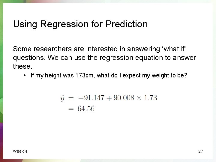
Using Regression for Prediction Some researchers are interested in answering ‘what if’ questions. We can use the regression equation to answer these. • If my height was 173 cm, what do I expect my weight to be? Week 4 27

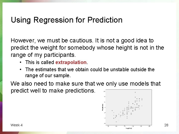
Using Regression for Prediction However, we must be cautious. It is not a good idea to predict the weight for somebody whose height is not in the range of my participants. • This is called extrapolation. • The estimates that we obtain could be unstable outside the range of our sample. We also need to make sure that we only use models that predict well to make predictions. Week 4 28

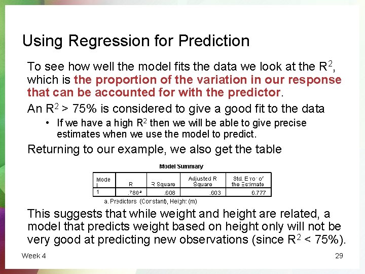
Using Regression for Prediction To see how well the model fits the data we look at the R 2, which is the proportion of the variation in our response that can be accounted for with the predictor. An R 2 > 75% is considered to give a good fit to the data • If we have a high R 2 then we will be able to give precise estimates when we use the model to predict. Returning to our example, we also get the table This suggests that while weight and height are related, a model that predicts weight based on height only will not be very good at predicting new observations (since R 2 < 75%). Week 4 29

GOOD LUCK IN THE ASSIGNMENT! UTS CRICOS PROVIDER CODE: 00099 F

Week 4 31