3 Structures and Strategies for State Space Search

3 Structures and Strategies for State Space Search 3. 0 Introduction 3. 1 Graph Theory 3. 2 Strategies for State Space Search 3. 3 Using the State Space to Represent Reasoning with the Predicate Calculus 3. 4 Epilogue and References 3. 5 Exercises Additional references for the slides: Russell and Norvig’s AI book. Robert Wilensky’s CS 188 slides: www. cs. berkeley. edu/%7 wilensky/cs 188/lectures/index. html 1

Chapter Objectives • Learn the basics of state space representation • Learn the basics of search in state space • The agent model: Has a problem, searches for a solution. 2

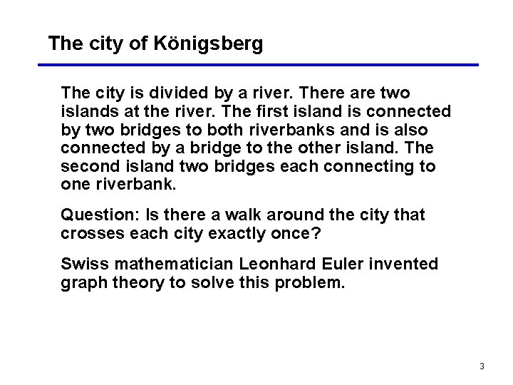
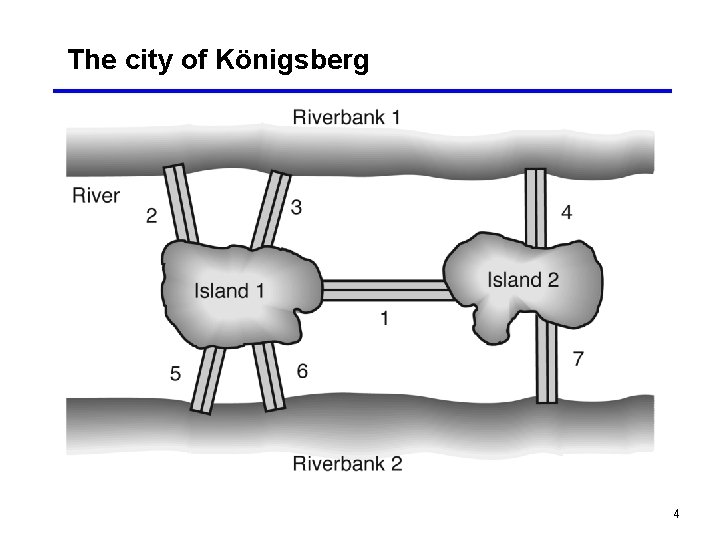
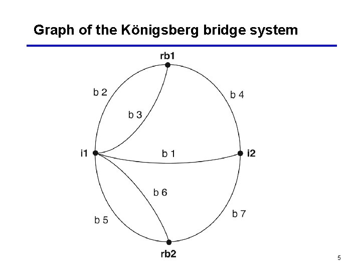
The city of Königsberg The city is divided by a river. There are two islands at the river. The first island is connected by two bridges to both riverbanks and is also connected by a bridge to the other island. The second island two bridges each connecting to one riverbank. Question: Is there a walk around the city that crosses each city exactly once? Swiss mathematician Leonhard Euler invented graph theory to solve this problem. 3

The city of Königsberg 4

Graph of the Königsberg bridge system 5

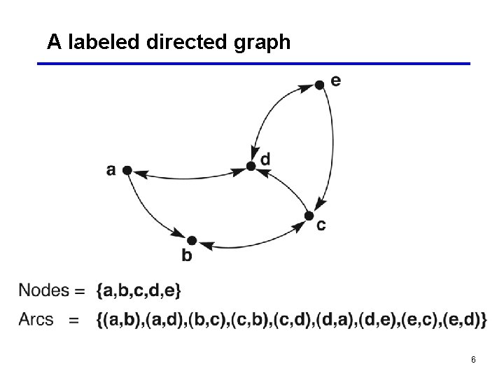
A labeled directed graph 6

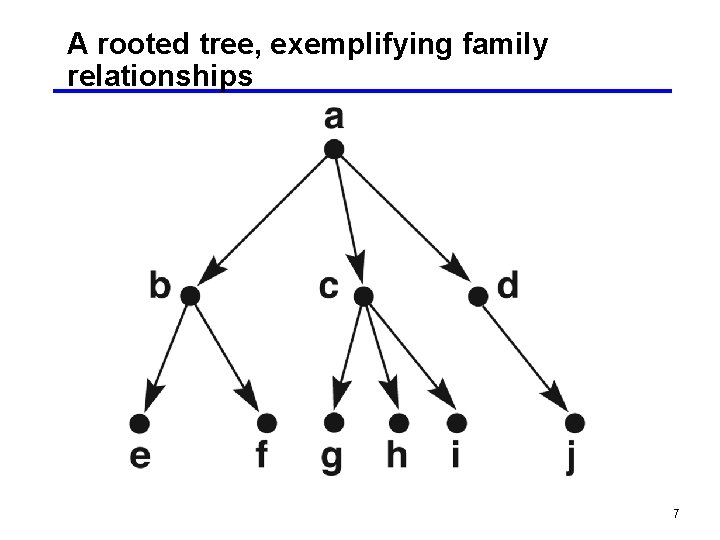
A rooted tree, exemplifying family relationships 7

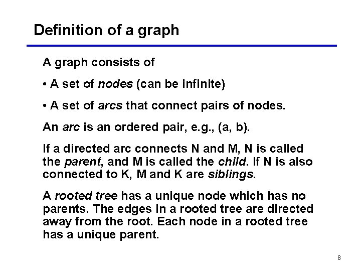
Definition of a graph A graph consists of • A set of nodes (can be infinite) • A set of arcs that connect pairs of nodes. An arc is an ordered pair, e. g. , (a, b). If a directed arc connects N and M, N is called the parent, and M is called the child. If N is also connected to K, M and K are siblings. A rooted tree has a unique node which has no parents. The edges in a rooted tree are directed away from the root. Each node in a rooted tree has a unique parent. 8

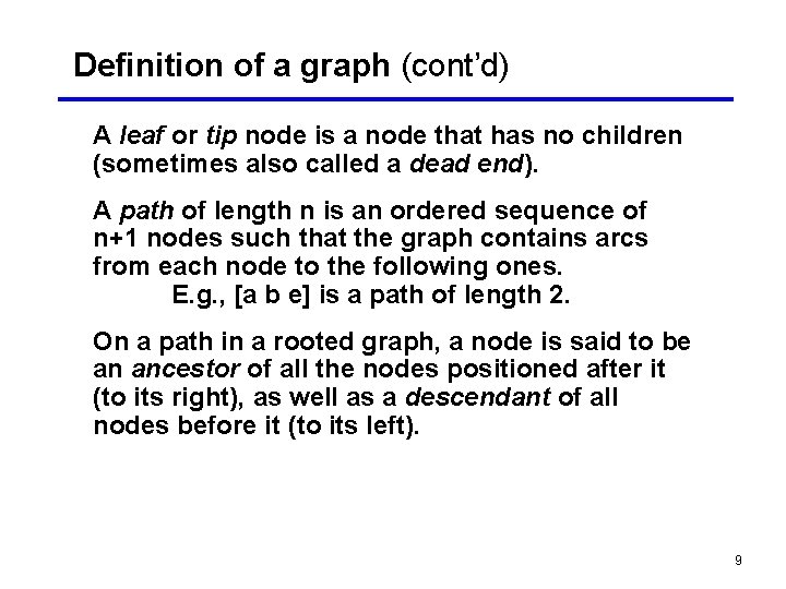
Definition of a graph (cont’d) A leaf or tip node is a node that has no children (sometimes also called a dead end). A path of length n is an ordered sequence of n+1 nodes such that the graph contains arcs from each node to the following ones. E. g. , [a b e] is a path of length 2. On a path in a rooted graph, a node is said to be an ancestor of all the nodes positioned after it (to its right), as well as a descendant of all nodes before it (to its left). 9

Definition of a graph (cont’d) A path that contains any node more than once is said to contain a cycle or loop. A tree is a graph in which there is a unique path between every pair of nodes. Two nodes are said to be connected if a path exists that includes them both. 10

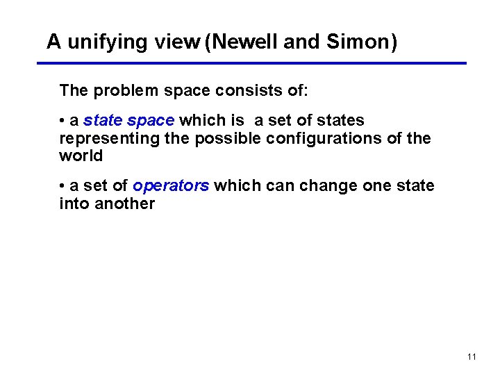
A unifying view (Newell and Simon) The problem space consists of: • a state space which is a set of states representing the possible configurations of the world • a set of operators which can change one state into another 11

State space search Represented by a four-tuple [N, A, S, GD], where: • N is the problem space • A is the set of arcs (or links) between nodes. These correspond to the operators. • S is a nonempty subset of N. It represents the start state(s) of the problem. • GD is a nonempty subset of N. It represents the goal state(s) of the problem. The states in GD are described using either: a measurable property of the states a property of the path developed in the search (a solution path is a path from node S to a node in GD ) 12

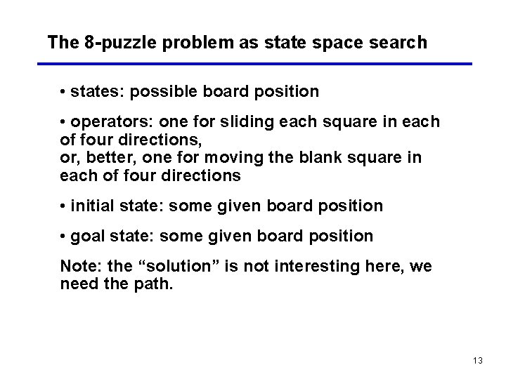
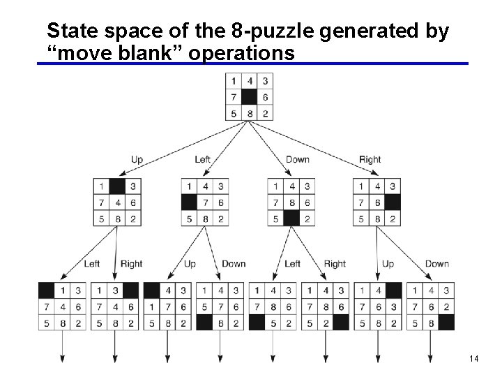
The 8 -puzzle problem as state space search • states: possible board position • operators: one for sliding each square in each of four directions, or, better, one for moving the blank square in each of four directions • initial state: some given board position • goal state: some given board position Note: the “solution” is not interesting here, we need the path. 13

State space of the 8 -puzzle generated by “move blank” operations 14

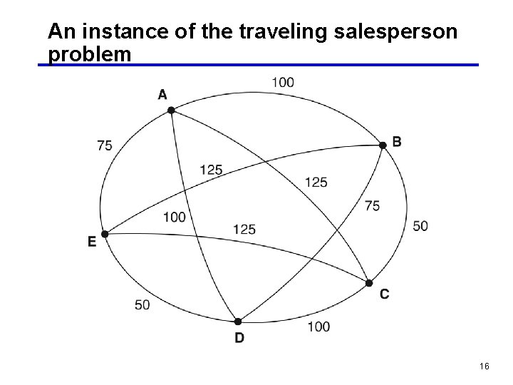
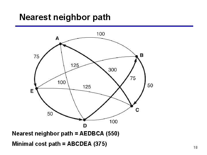
Traveling salesperson problem as state space search The salesperson has n cities to visit and must then return home. Find the shortest path to travel. • state space • operators: • initial state: • goal state: Note: this is a “two-player” game 15

An instance of the traveling salesperson problem 16

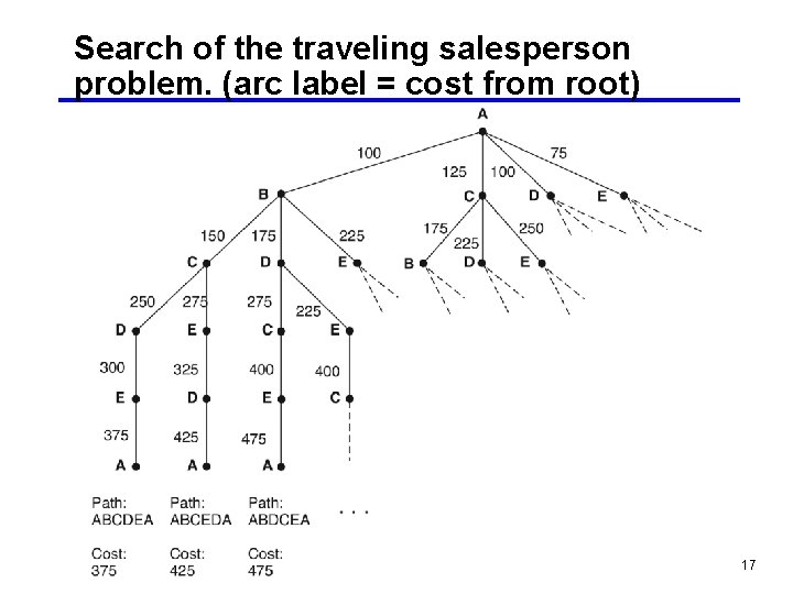
Search of the traveling salesperson problem. (arc label = cost from root) 17

Nearest neighbor path = AEDBCA (550) Minimal cost path = ABCDEA (375) 18

Tic-tac-toe as state space search • states: • operators: • initial state: • goal state: Note: this is a “two-player” game 19

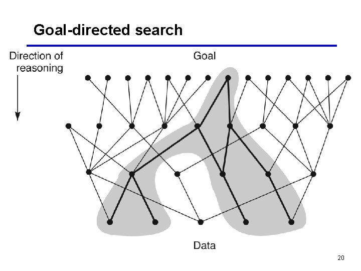
Goal-directed search 20

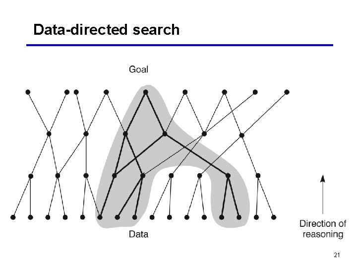
Data-directed search 21

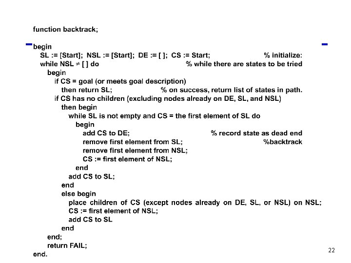
22

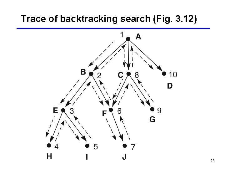
Trace of backtracking search (Fig. 3. 12) 23

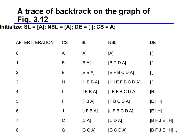
A trace of backtrack on the graph of Fig. 3. 12 24

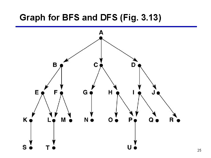
Graph for BFS and DFS (Fig. 3. 13) 25

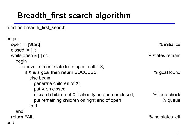
Breadth_first search algorithm 26

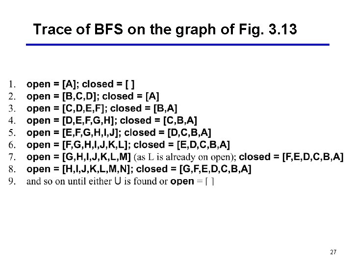
Trace of BFS on the graph of Fig. 3. 13 27

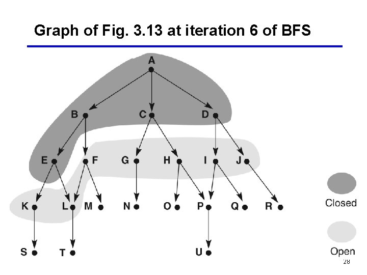
Graph of Fig. 3. 13 at iteration 6 of BFS 28

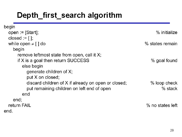
Depth_first_search algorithm 29

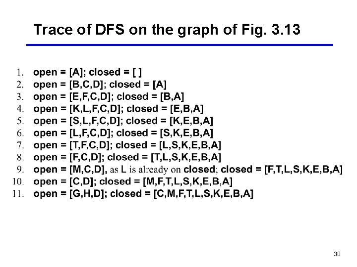
Trace of DFS on the graph of Fig. 3. 13 30

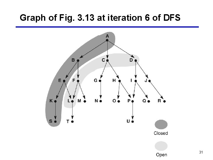
Graph of Fig. 3. 13 at iteration 6 of DFS 31

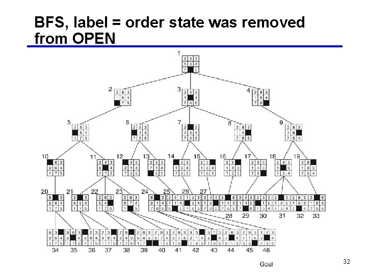
BFS, label = order state was removed from OPEN 32

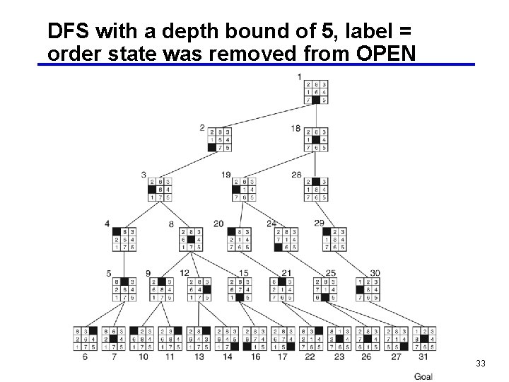
DFS with a depth bound of 5, label = order state was removed from OPEN 33