3 Linear Regression and Least Squares Method 1

(3) Linear Regression and Least Squares Method 1

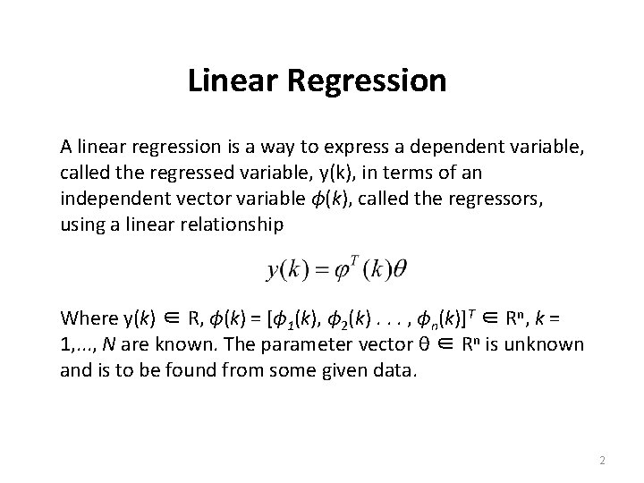
Linear Regression A linear regression is a way to express a dependent variable, called the regressed variable, y(k), in terms of an independent vector variable ϕ(k), called the regressors, using a linear relationship Where y(k) ∈ R, ϕ(k) = [ϕ 1(k), ϕ 2(k). . . , ϕn(k)]T ∈ Rn, k = 1, . . . , N are known. The parameter vector θ ∈ Rn is unknown and is to be found from some given data. 2

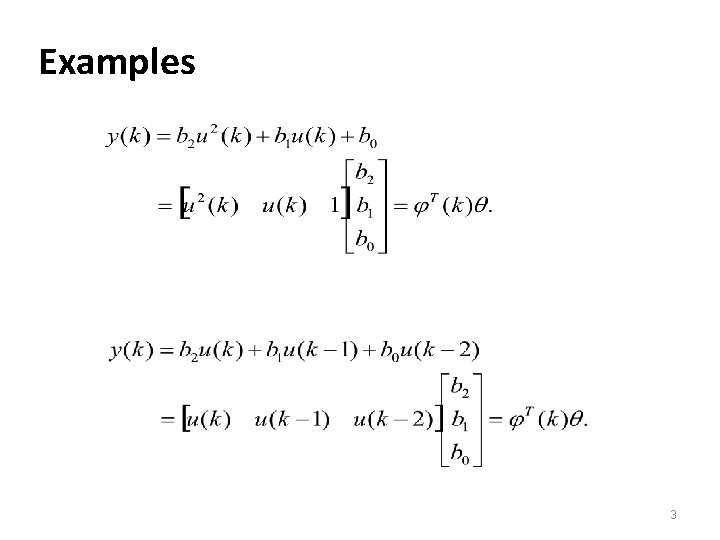
Examples 3

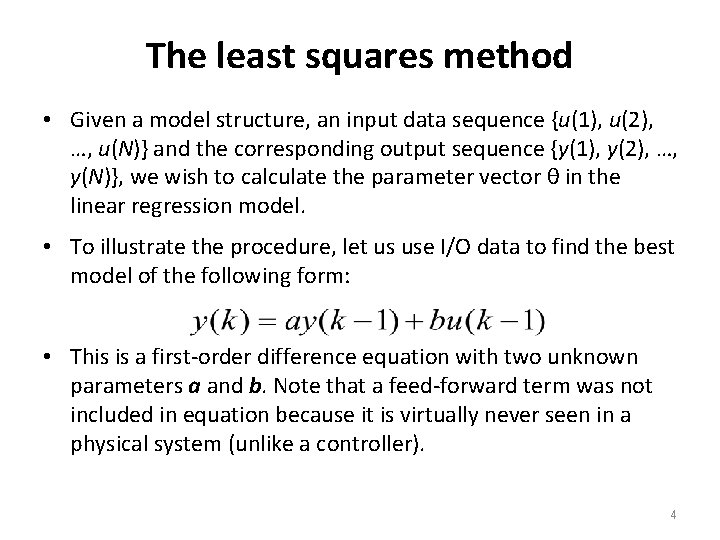
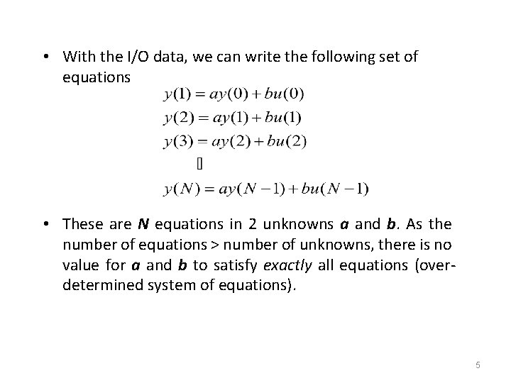
The least squares method • Given a model structure, an input data sequence {u(1), u(2), …, u(N)} and the corresponding output sequence {y(1), y(2), …, y(N)}, we wish to calculate the parameter vector θ in the linear regression model. • To illustrate the procedure, let us use I/O data to find the best model of the following form: • This is a first-order difference equation with two unknown parameters a and b. Note that a feed-forward term was not included in equation because it is virtually never seen in a physical system (unlike a controller). 4

• With the I/O data, we can write the following set of equations • These are N equations in 2 unknowns a and b. As the number of equations > number of unknowns, there is no value for a and b to satisfy exactly all equations (overdetermined system of equations). 5

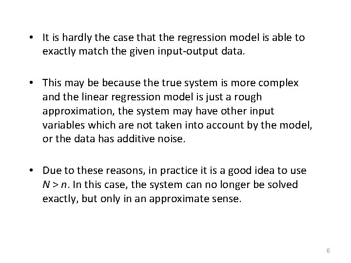
• It is hardly the case that the regression model is able to exactly match the given input-output data. • This may be because the true system is more complex and the linear regression model is just a rough approximation, the system may have other input variables which are not taken into account by the model, or the data has additive noise. • Due to these reasons, in practice it is a good idea to use N > n. In this case, the system can no longer be solved exactly, but only in an approximate sense. 6

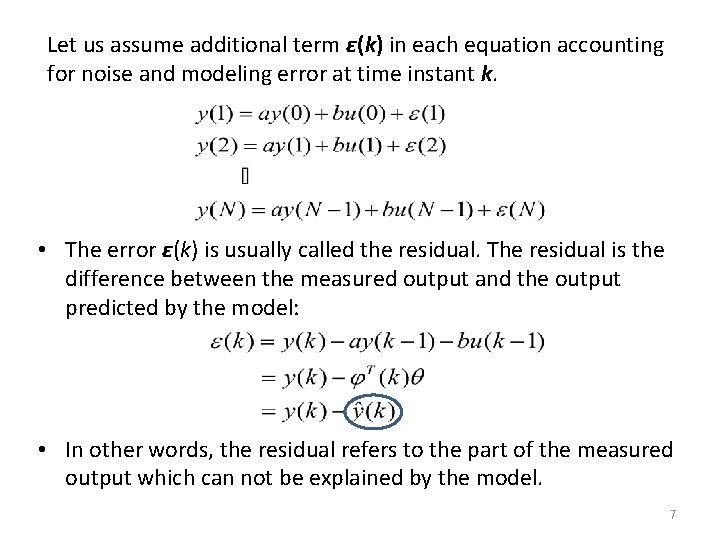
Let us assume additional term ε(k) in each equation accounting for noise and modeling error at time instant k. • The error ε(k) is usually called the residual. The residual is the difference between the measured output and the output predicted by the model: • In other words, the residual refers to the part of the measured output which can not be explained by the model. 7

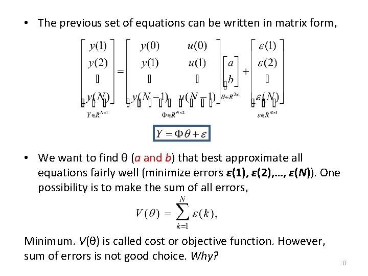
• The previous set of equations can be written in matrix form, • We want to find θ (a and b) that best approximate all equations fairly well (minimize errors ε(1), ε(2), …, ε(N)). One possibility is to make the sum of all errors, Minimum. V(θ) is called cost or objective function. However, sum of errors is not good choice. Why? 8

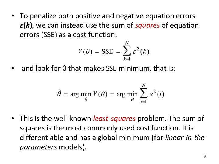
• To penalize both positive and negative equation errors ε(k), we can instead use the sum of squares of equation errors (SSE) as a cost function: • and look for θ that makes SSE minimum, that is: • This is the well-known least-squares problem. The sum of squares is the most commonly used cost function. It is differentiable and has a global minimum (for linear-in-theparameters models). 9

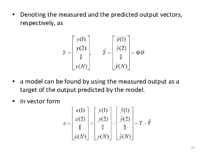
• Denoting the measured and the predicted output vectors, respectively, as • a model can be found by using the measured output as a target of the output predicted by the model. • In vector form 10

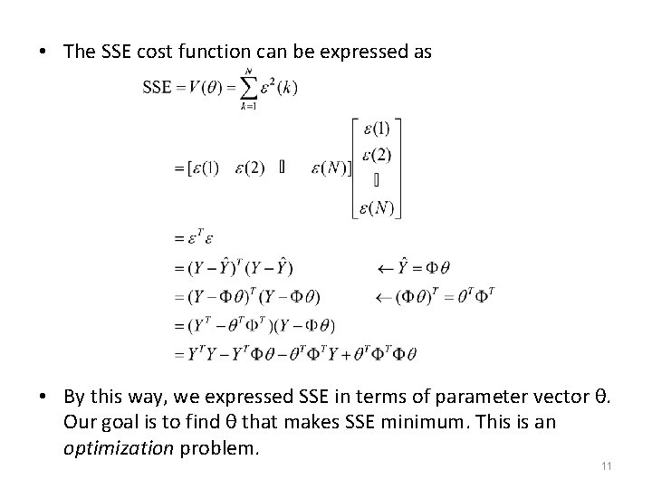
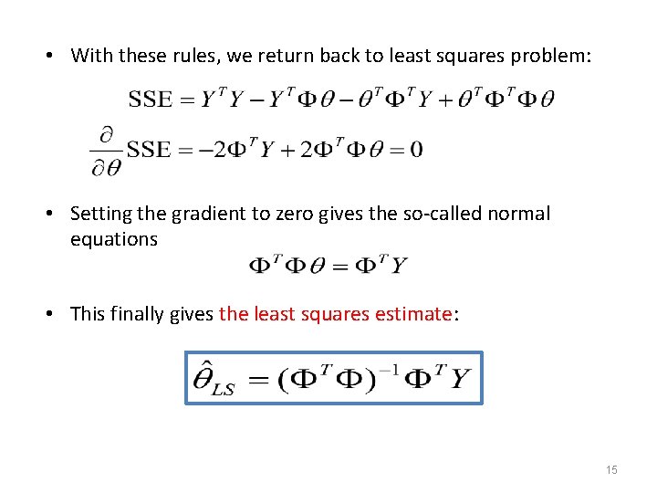
• The SSE cost function can be expressed as • By this way, we expressed SSE in terms of parameter vector θ. Our goal is to find θ that makes SSE minimum. This is an optimization problem. 11

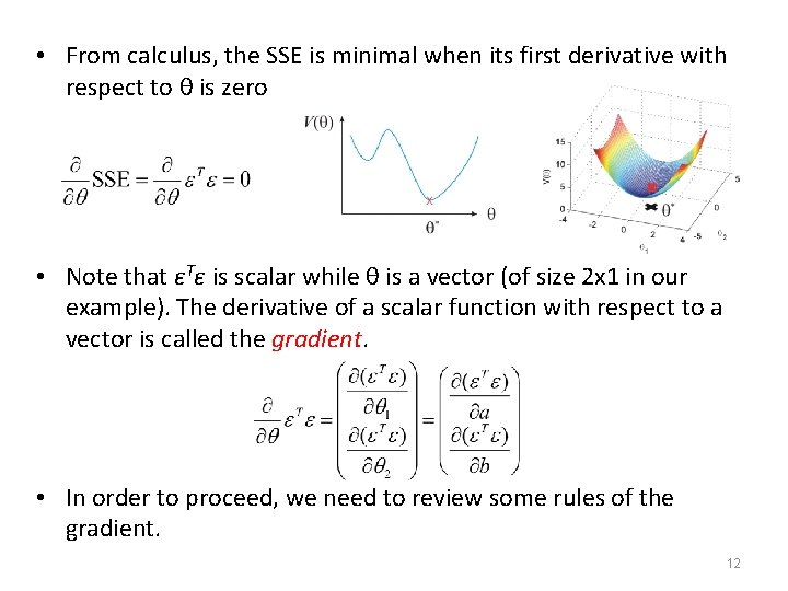
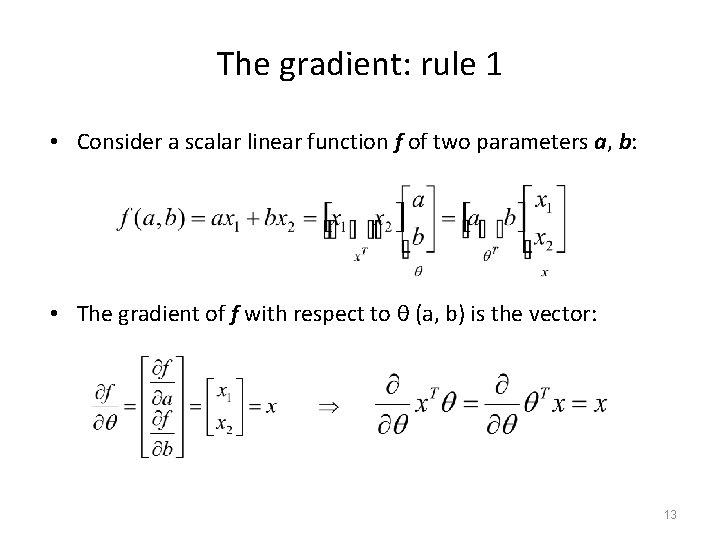
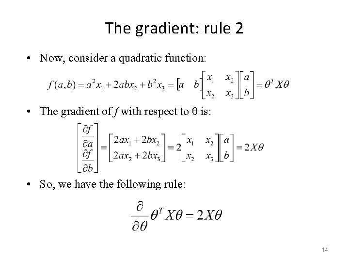
• From calculus, the SSE is minimal when its first derivative with respect to θ is zero • Note that εTε is scalar while θ is a vector (of size 2 x 1 in our example). The derivative of a scalar function with respect to a vector is called the gradient. • In order to proceed, we need to review some rules of the gradient. 12

The gradient: rule 1 • Consider a scalar linear function f of two parameters a, b: • The gradient of f with respect to θ (a, b) is the vector: 13

The gradient: rule 2 • Now, consider a quadratic function: • The gradient of f with respect to θ is: • So, we have the following rule: 14

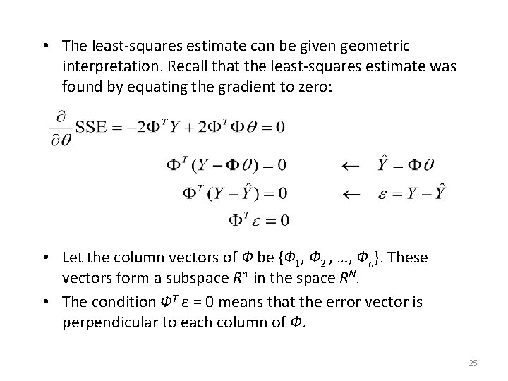
• With these rules, we return back to least squares problem: • Setting the gradient to zero gives the so-called normal equations • This finally gives the least squares estimate: 15

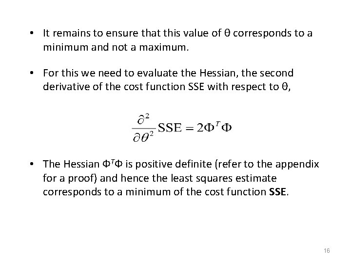
• It remains to ensure that this value of θ corresponds to a minimum and not a maximum. • For this we need to evaluate the Hessian, the second derivative of the cost function SSE with respect to θ, • The Hessian ФTФ is positive definite (refer to the appendix for a proof) and hence the least squares estimate corresponds to a minimum of the cost function SSE. 16

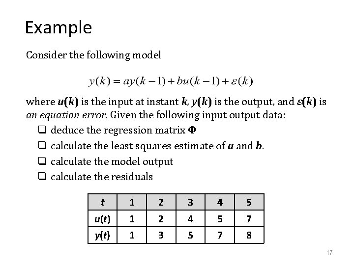
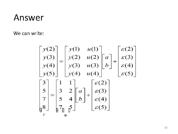
Example Consider the following model where u(k) is the input at instant k, y(k) is the output, and ε(k) is an equation error. Given the following input output data: q deduce the regression matrix Φ q calculate the least squares estimate of a and b. q calculate the model output q calculate the residuals t 1 2 3 4 5 u(t) 1 2 4 5 7 y(t) 1 3 5 7 8 17

Answer We can write: 18

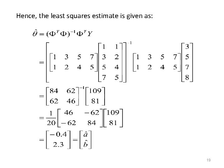
Hence, the least squares estimate is given as: 19

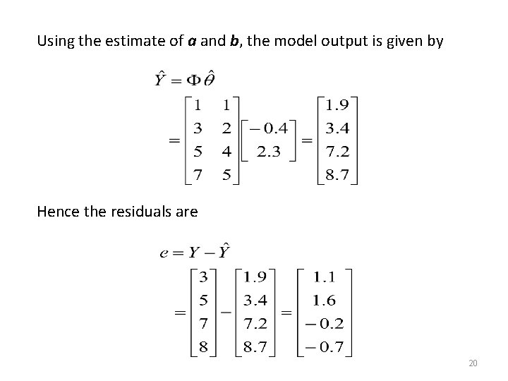
Using the estimate of a and b, the model output is given by Hence the residuals are 20

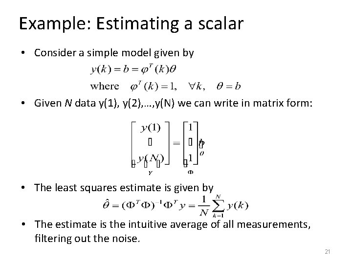
Example: Estimating a scalar • Consider a simple model given by • Given N data y(1), y(2), …, y(N) we can write in matrix form: • The least squares estimate is given by • The estimate is the intuitive average of all measurements, filtering out the noise. 21

Note on model order selection • The choice of the model order (i. e. the number of parameters) is up to the designer. • The designer may perform multiple fits with different orders and select the lowest order fit that yields acceptable agreement. • Selecting a model of too-high order means that you use the “extra” parameters to fit noise in the data. 22

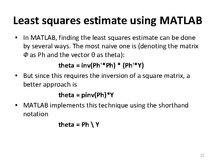
Least squares estimate using MATLAB • In MATLAB, finding the least squares estimate can be done by several ways. The most naive one is (denoting the matrix Ф as Ph and the vector θ as theta): theta = inv(Ph'*Ph) * (Ph'*Y) • But since this requires the inversion of a square matrix, a better approach is theta = pinv(Ph)*Y • MATLAB implements this technique using the shorthand notation theta = Ph Y 23

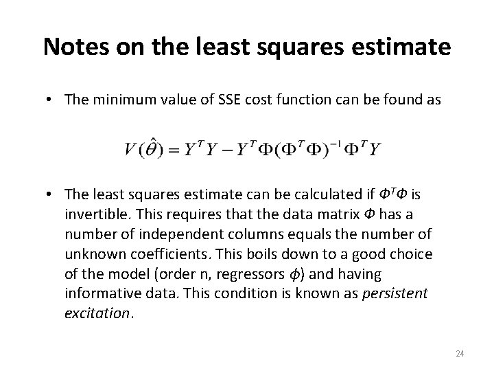
Notes on the least squares estimate • The minimum value of SSE cost function can be found as • The least squares estimate can be calculated if ФTФ is invertible. This requires that the data matrix Ф has a number of independent columns equals the number of unknown coefficients. This boils down to a good choice of the model (order n, regressors ϕ) and having informative data. This condition is known as persistent excitation. 24

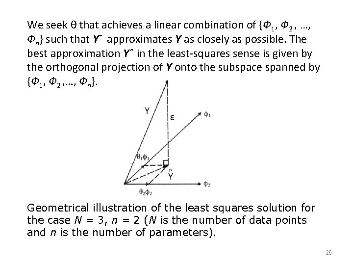
• The least-squares estimate can be given geometric interpretation. Recall that the least-squares estimate was found by equating the gradient to zero: • Let the column vectors of Ф be {Ф 1, Ф 2 , …, Фn}. These vectors form a subspace Rn in the space RN. • The condition ФT ε = 0 means that the error vector is perpendicular to each column of Ф. 25

We seek θ that achieves a linear combination of {Ф 1, Ф 2 , …, Фn} such that Yˆ approximates Y as closely as possible. The best approximation Yˆ in the least-squares sense is given by the orthogonal projection of Y onto the subspace spanned by {Ф 1, Ф 2 , …, Фn}. Geometrical illustration of the least squares solution for the case N = 3, n = 2 (N is the number of data points and n is the number of parameters). 26

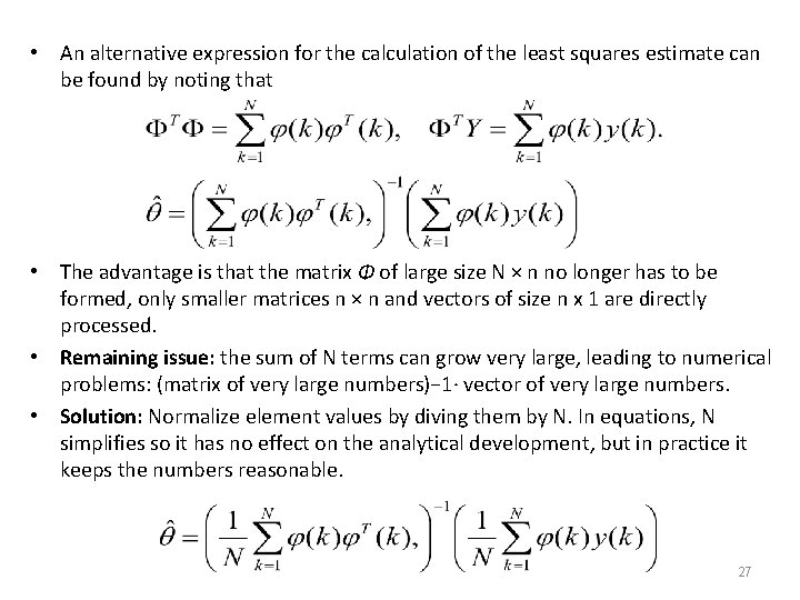
• An alternative expression for the calculation of the least squares estimate can be found by noting that • The advantage is that the matrix Φ of large size N × n no longer has to be formed, only smaller matrices n × n and vectors of size n x 1 are directly processed. • Remaining issue: the sum of N terms can grow very large, leading to numerical problems: (matrix of very large numbers)− 1· vector of very large numbers. • Solution: Normalize element values by diving them by N. In equations, N simplifies so it has no effect on the analytical development, but in practice it keeps the numbers reasonable. 27

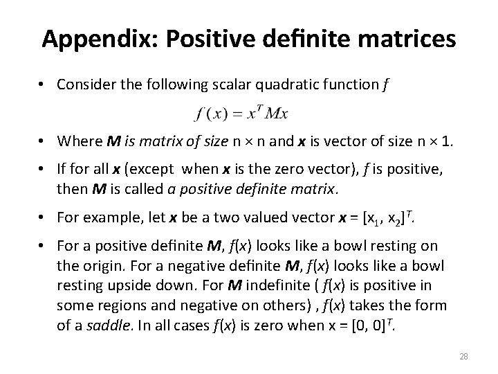
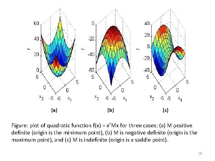
Appendix: Positive definite matrices • Consider the following scalar quadratic function f • Where M is matrix of size n × n and x is vector of size n × 1. • If for all x (except when x is the zero vector), f is positive, then M is called a positive definite matrix. • For example, let x be a two valued vector x = [x 1, x 2]T. • For a positive definite M, f(x) looks like a bowl resting on the origin. For a negative definite M, f(x) looks like a bowl resting upside down. For M indefinite ( f(x) is positive in some regions and negative on others) , f(x) takes the form of a saddle. In all cases f(x) is zero when x = [0, 0]T. 28

(a) (b) (c) Figure: plot of quadratic function f(x) = x. TMx for three cases: (a) M positive definite (origin is the minimum point), (b) M is negative definite (origin is the maximum point), and (c) M is indefinite (origin is a saddle point). 29

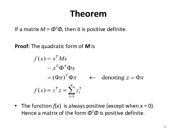
Theorem If a matrix M = ΦTΦ, then it is positive definite. Proof: The quadratic form of M is • The function f(x) is always positive (except when x = 0). Hence a matrix of the form ΦTΦ is positive definite. 30