3 D SUBMILLIMETER SPECTROSCOPY FOR ASTROPHYSICS AND SPECTRAL

3 -D SUBMILLIMETER SPECTROSCOPY FOR ASTROPHYSICS AND SPECTRAL ASSIGNMENT SARAH M. FORTMAN, IVAN R. MEDVEDEV, FRANK C. DE LUCIA, Department of Physics, The Ohio State University, Columbus, OH 43210 -1106, USA. OSU International Symposium on Molecular Spectroscopy Columbus, OH June 16 th, 2008

Two Related Objectives courtesy of J. Cernicharo Spectroscopy Challenge • Bootstrap Assignment in Complex Spectra • FASSST spectra may contain >10^5 lines in many vibrational states Traditional Approach • Use 2 D (intensity, frequency) spectra to assign and bootstrap in each vibrational state New Approach • Observe intensity calibrated variable temperature spectrum and calculate lower state energies. • Use intensity, frequency and lower state energies in the bootstrap assignment Intensity Calibrated Variable Temperature Spectroscopy • Observe 2 D spectra at many temperatures • Calculate intensity, frequency and lower state energies for assigned and unassigned lines • Give astronomers what they want • Give spectroscopists more information Astronomy Challenge • Current telescopes approach confusion limit • Many unassigned lines • New systems (Alma, Herschel) will be more powerful Traditional Approach • Quantum Mechanical predictions of astrophysical spectra give intensity and frequency as a function of temperature • Spectroscopists calculate and fit what we can, not what astronomers need New Approach • Predict intensity and frequency as a function of temperature without assignment

Spectroscopic Challenge Predicted lines from SPFIT. cat file FREQ 222205. 8884 222206. 5102 222216. 2472 222222. 2687 222662. 1685 222662. 5968 222665. 1993 222696. 0695 222725. 9166 222746. 5775 222800. 4652 222821. 1262 ERR 0. 0141 0. 0142 0. 0128 0. 0241 0. 1481 0. 0071 0. 1573 0. 0098 0. 1222 0. 1175 0. 1143 0. 1312 LGINT -7. 0138 -6. 1572 -7. 3542 -7. 8356 -6. 0426 -7. 8356 -6. 7291 -7. 8669 -8. 1094 -8. 1092 -7. 8664 DR ELO GUP TAG QNFMT QN’ 3 1502. 8669 81 630061404402218 3 1502. 8675 81 630061404402318 3 916. 1480 21 63006140410 8 2 3 1502. 8669 81 630061404402318 3 2033. 0142109 630061404543718 3 915. 3357 21 63006140410 7 3 3 2033. 0133109 630061404543618 3 900. 5161 17 630061404 8 6 2 3 1956. 8275105 630061404523319 3 1956. 8268105 630061404523319 3 1956. 8275105 630061404523419 3 1956. 8268105 630061404523419 Fitted Constants from SPFIT. fit file 1 1 0 0 0 0 1 1 QN” 402119 402219 9 8 1 402119 543619 9 7 2 543519 7 4 3 523320 523220 1 1 0 0 0 0 1 1 1 910099 2 0 3 10000 4 20000 5 30000 6 610000 7 610100 8 611000 9 610200 10 612000 11 100000 12 1000000100 NEW PARAMETER (EST. ERROR) 1. 468190000( 0) 0. 00000 26355017. 840800( 0) 0. 000000 12962. 3189(307) 0. 0000 12085. 7215(308) -0. 0000 6242. 05887( 35) 0. 00000 -196. 061( 69) 0. 000 2. 464( 33)E-03 -0. 000 E-03 -2. 3201(144)E-03 -0. 0000 E-03 -0. 0928( 48)E-06 -0. 0000 E-06 -0. 06750(269)E-06 -0. 00000 E-06 -17. 7136( 60) -0. 0000 -0. 4134(150)E-03 0. 0000 E-03
 Intensity (nm 2*MHz) Lower State Energy")
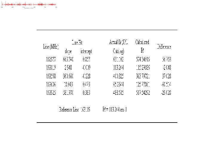
Graphing in Two and Three Dimensions Frequency (MHz) Intensity (nm 2*MHz) Lower State Energy (cm-1) 162977 5. 1963711 631. 1015 163119 17. 025509 113. 2438 163568 5. 0442872 400. 8251 163606 37. 162086 65. 264397 163925 4. 3062572 488. 5152 • Traditional approach uses a 2 D (intensity vs. frequency) plot • New approach creates a 3 D plot from the intensity, frequency and lower state energy data
 spectrometer Mylar beam splitter 1 Thermal enclosure Lens")
FAst Scan Submillimeter Spectroscopic Technique (FASSST) spectrometer Mylar beam splitter 1 Thermal enclosure Lens Reference gas cell BWO Path of microwave radiation Mylar beam splitter 2 Aluminum cell: length 6 m; Length ~60 cm diameter 15 cm Glass rings used to suppress reflections In. Sb detector 2 Reference channel Preamplifier Interference fringes Spectrum Stepper motor Signal channel Lens In. Sb detector 1 Frequency roll-off preamplifier Magnet Ring cavity: L~15 m Data acquisition system Computer Stainless steel rails Slow wave structure sweeper Filament voltage power supply High voltage power supply Trigger channel /Triangular waveform channel

Temperature Control • • • Ran experiment once Temperature Range: 228 – 405 K (-45 – 132 °C) at ~. 8 degrees/min Took 700 scans over 3. 5 hours totaling 29. 6 GB of data

Spectra as a Function of Temperature • The physical basis of the calculation of the lower state energy is the differential change in line strength with temperature. Subset of Data (in total experiment 700 traces over 50 GHz)

Ratios to Obtain Lower State Energy Consider taking the ratio of two lines of which one is assigned and the other is unassigned. We can plot the log of the ratio in log(1/T) space and expect to see a straight line. • Scatter from the peak finder • Ripples (variation in reflection with T? ) • Temperature calibration (currently thermocouples, starting to use spectroscopic temperature)

Lower State Energy vs. Thermal Behavior Okay but not great

Propagation of Error and Uncertainties Astronomy Spectroscopy We expect to reduce uncertainties by a factor of 10 by: • Replacing the peak finder with analysis • Fitting a model to the baseline ripple • Using a grand fit of all assigned lines as the reference line instead of a single line • Getting a proper average over the ends by using the spectroscopic temperature • Operating over a larger temperature range (using a collisional cooling cell to 2 K) • • The smallest errors in intensities will come when the calculated temperature is bounded by experimental temperatures The error in the predicted intensity will be of the order the error in the observations (or better because we make many observations).

- Slides: 12