
3 D Mathematics CIS 488588 Bruce R Maxim
3 D Mathematics CIS 488/588 Bruce R. Maxim UM-Dearborn 12/1/2020 1
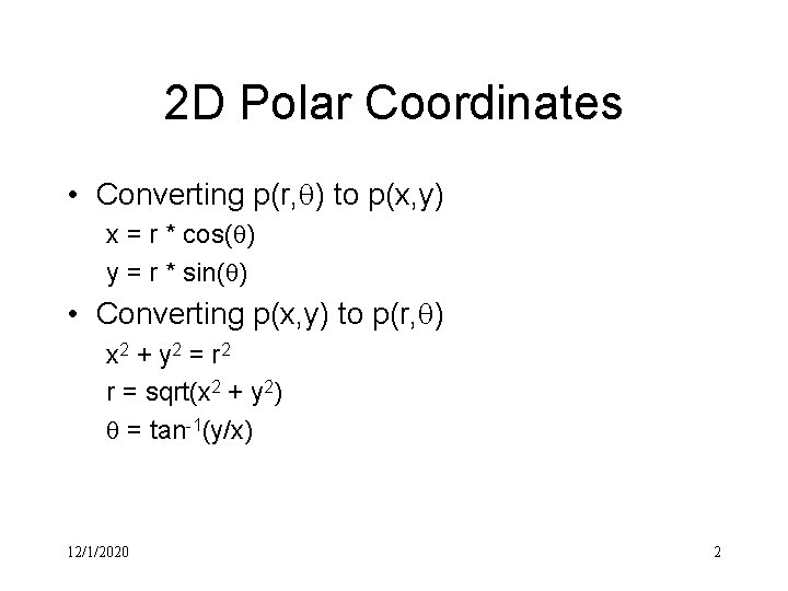
2 D Polar Coordinates • Converting p(r, ) to p(x, y) x = r * cos( ) y = r * sin( ) • Converting p(x, y) to p(r, ) x 2 + y 2 = r 2 r = sqrt(x 2 + y 2) = tan-1(y/x) 12/1/2020 2
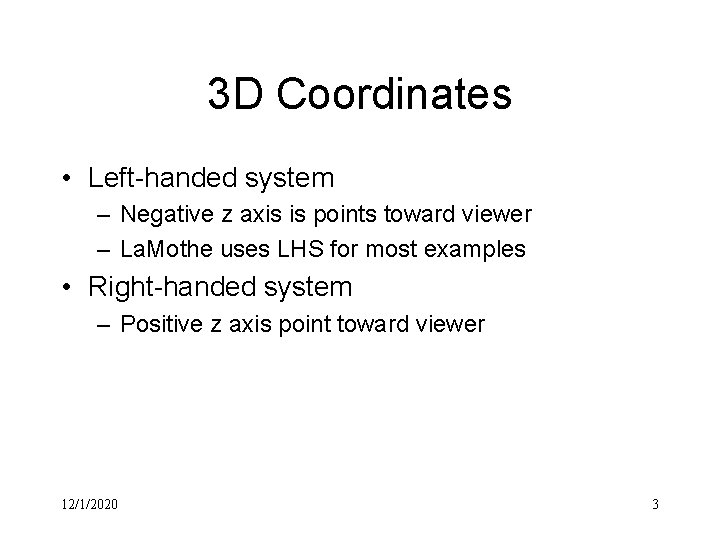
3 D Coordinates • Left-handed system – Negative z axis is points toward viewer – La. Mothe uses LHS for most examples • Right-handed system – Positive z axis point toward viewer 12/1/2020 3
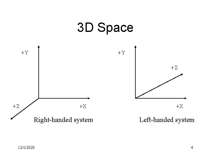
3 D Space +Y +Y +Z +Z +X Right-handed system 12/1/2020 +X Left-handed system 4
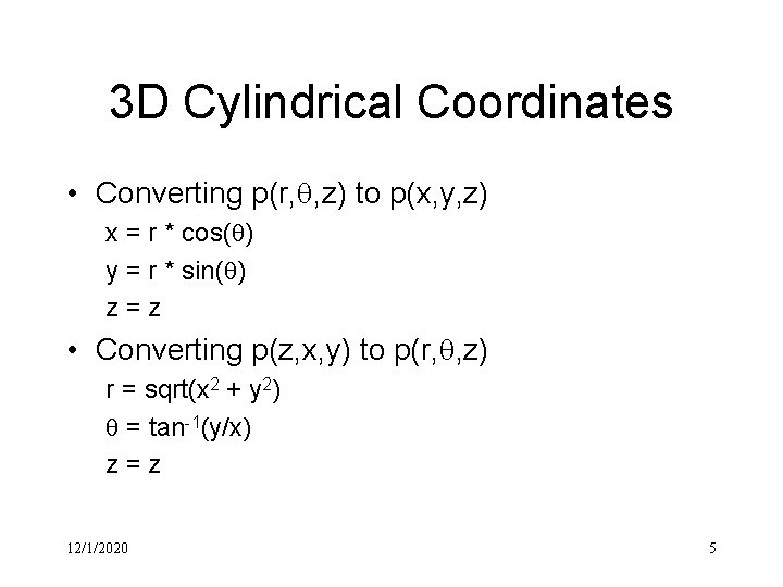
3 D Cylindrical Coordinates • Converting p(r, , z) to p(x, y, z) x = r * cos( ) y = r * sin( ) z=z • Converting p(z, x, y) to p(r, , z) r = sqrt(x 2 + y 2) = tan-1(y/x) z=z 12/1/2020 5
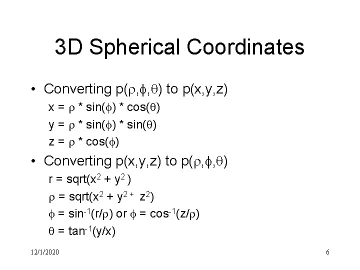
3 D Spherical Coordinates • Converting p( , , ) to p(x, y, z) x = * sin( ) * cos( ) y = * sin( ) z = * cos( ) • Converting p(x, y, z) to p( , , ) r = sqrt(x 2 + y 2 ) = sqrt(x 2 + y 2 + z 2) = sin-1(r/ ) or = cos-1(z/ ) = tan-1(y/x) 12/1/2020 6
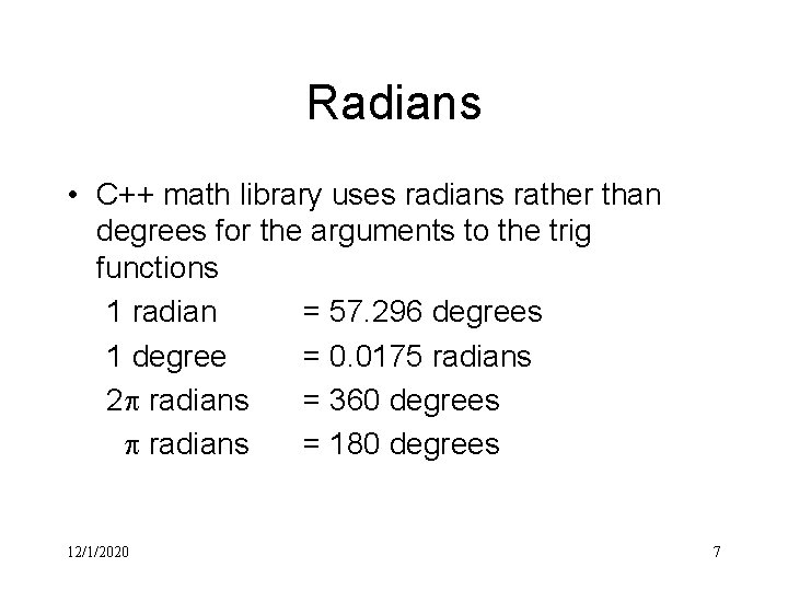
Radians • C++ math library uses radians rather than degrees for the arguments to the trig functions 1 radian = 57. 296 degrees 1 degree = 0. 0175 radians 2 radians = 360 degrees radians = 180 degrees 12/1/2020 7
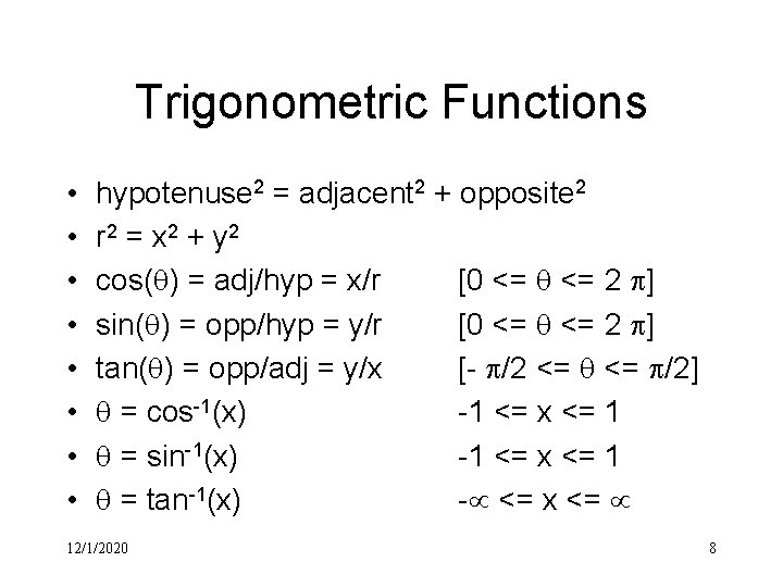
Trigonometric Functions • • hypotenuse 2 = adjacent 2 + opposite 2 r 2 = x 2 + y 2 cos( ) = adj/hyp = x/r [0 <= 2 ] sin( ) = opp/hyp = y/r [0 <= 2 ] tan( ) = opp/adj = y/x [- /2 <= /2] = cos-1(x) -1 <= x <= 1 = sin-1(x) -1 <= x <= 1 = tan-1(x) - <= x <= 12/1/2020 8
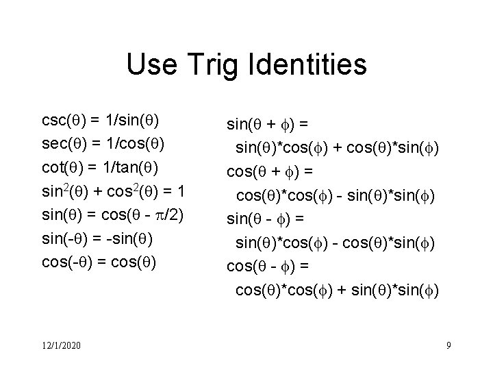
Use Trig Identities csc( ) = 1/sin( ) sec( ) = 1/cos( ) cot( ) = 1/tan( ) sin 2( ) + cos 2( ) = 1 sin( ) = cos( - /2) sin(- ) = -sin( ) cos(- ) = cos( ) 12/1/2020 sin( + ) = sin( )*cos( ) + cos( )*sin( ) cos( + ) = cos( )*cos( ) - sin( )*sin( ) sin( - ) = sin( )*cos( ) - cos( )*sin( ) cos( - ) = cos( )*cos( ) + sin( )*sin( ) 9
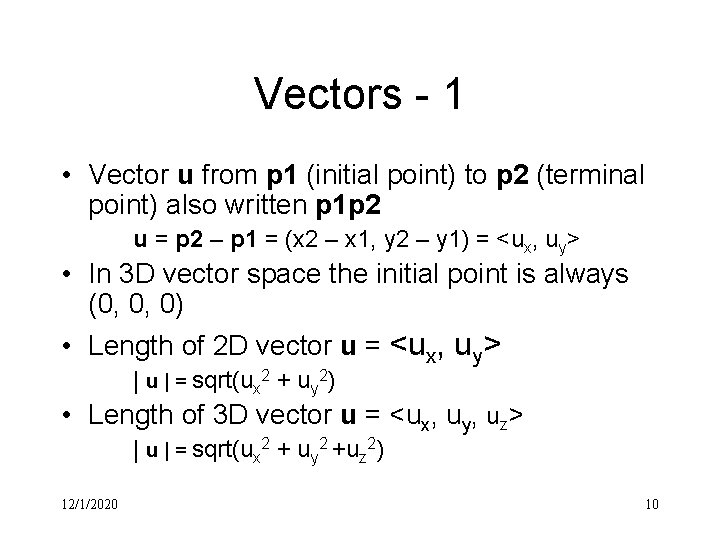
Vectors - 1 • Vector u from p 1 (initial point) to p 2 (terminal point) also written p 1 p 2 u = p 2 – p 1 = (x 2 – x 1, y 2 – y 1) = <ux, uy> • In 3 D vector space the initial point is always (0, 0, 0) • Length of 2 D vector u = <ux, uy> | u | = sqrt(ux 2 + uy 2) • Length of 3 D vector u = <ux, uy, uz> | u | = sqrt(ux 2 + uy 2 +uz 2) 12/1/2020 10
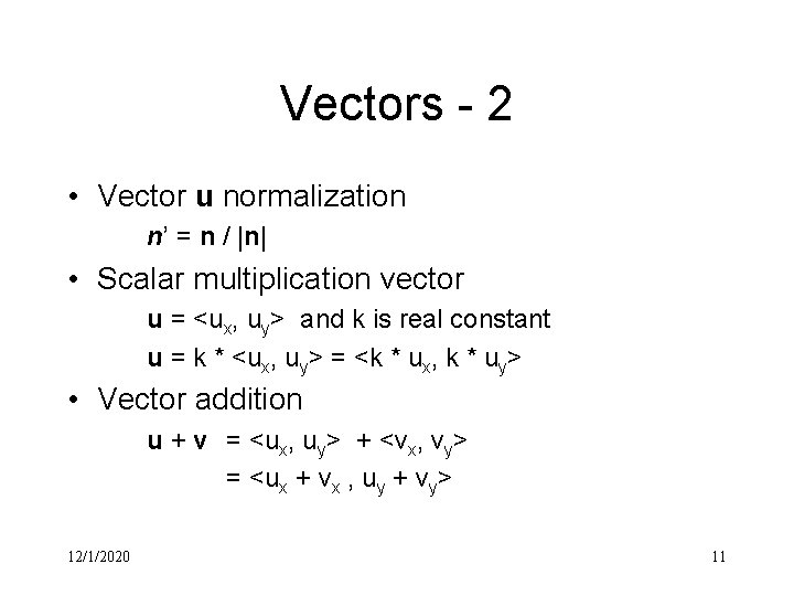
Vectors - 2 • Vector u normalization n’ = n / |n| • Scalar multiplication vector u = <ux, uy> and k is real constant u = k * <ux, uy> = <k * ux, k * uy> • Vector addition u + v = <ux, uy> + <vx, vy> = <ux + vx , uy + vy> 12/1/2020 11
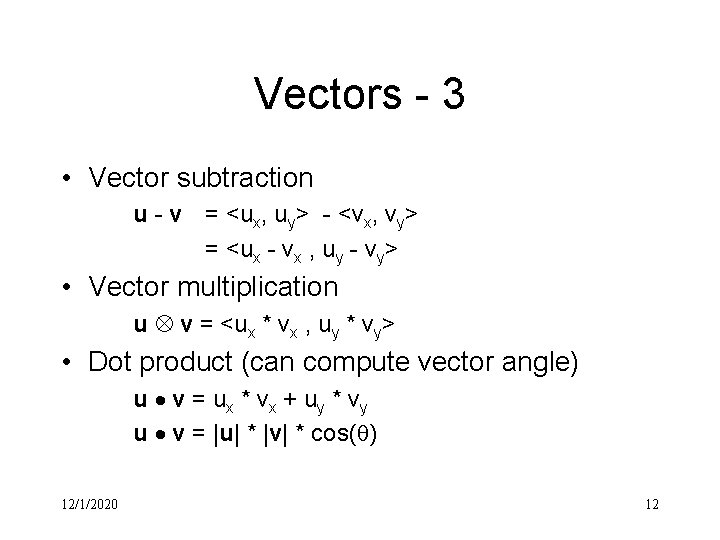
Vectors - 3 • Vector subtraction u - v = <ux, uy> - <vx, vy> = <ux - vx , uy - vy> • Vector multiplication u v = <ux * vx , uy * vy> • Dot product (can compute vector angle) u v = ux * vx + uy * vy u v = |u| * |v| * cos( ) 12/1/2020 12
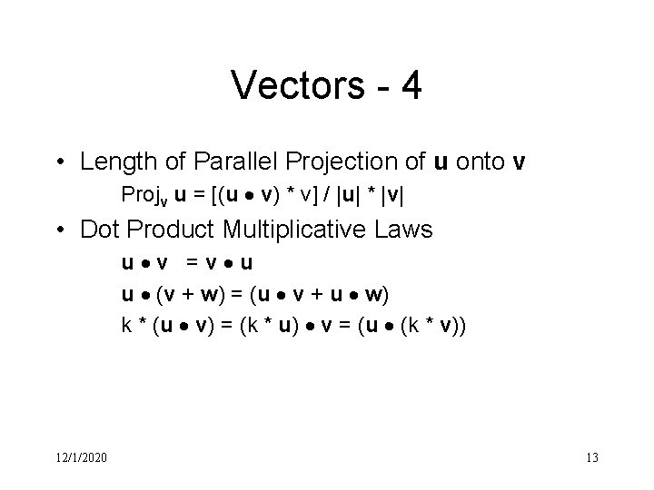
Vectors - 4 • Length of Parallel Projection of u onto v Projv u = [(u v) * v] / |u| * |v| • Dot Product Multiplicative Laws u v =v u u (v + w) = (u v + u w) k * (u v) = (k * u) v = (u (k * v)) 12/1/2020 13

Vectors - 5 • Cross Product u x v = |u| * |v| * sin( ) * n • Cross Product Multiplication Laws u x v = -(v x u) u x (v + w) = (u x v) + (u x w) (u + v) x w = (u x w) + (v x w) k * (u x v) = (k * u) x v = u x (k * v) 12/1/2020 14
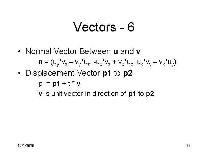
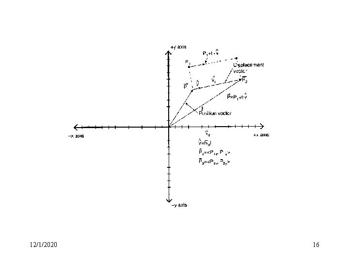
Vectors - 6 • Normal Vector Between u and v n = (uy*vz – vy*uz, -ux*vz + vx*uz, ux*vy – vx*uy) • Displacement Vector p 1 to p 2 p = p 1 + t * v v is unit vector in direction of p 1 to p 2 12/1/2020 15
12/1/2020 16
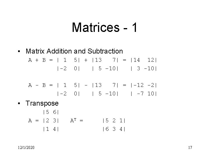
Matrices - 1 • Matrix Addition and Subtraction A + B = | 1 |-2 5| + |13 7| = |14 12| 0| | 5 – 10| | 3 -10| A - B = | 1 |-2 5| - |13 7| = |-12 -2| 0| | 5 – 10| | -7 10| • Transpose |5 6| A = |2 3| |1 4| 12/1/2020 AT = |5 2 1| |6 3 4| 17
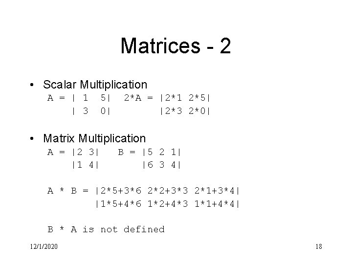
Matrices - 2 • Scalar Multiplication A = | 1 | 3 5| 0| 2*A = |2*1 2*5| |2*3 2*0| • Matrix Multiplication A = |2 3| |1 4| B = |5 2 1| |6 3 4| A * B = |2*5+3*6 2*2+3*3 2*1+3*4| |1*5+4*6 1*2+4*3 1*1+4*4| B * A is not defined 12/1/2020 18
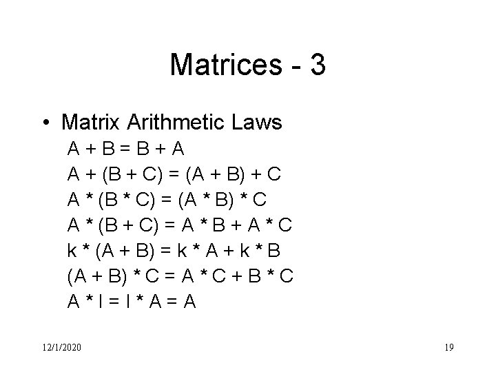
Matrices - 3 • Matrix Arithmetic Laws A+B=B+A A + (B + C) = (A + B) + C A * (B * C) = (A * B) * C A * (B + C) = A * B + A * C k * (A + B) = k * A + k * B (A + B) * C = A * C + B * C A*I=I*A=A 12/1/2020 19
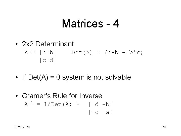
Matrices - 4 • 2 x 2 Determinant A = |a b| |c d| Det(A) = (a*b – b*c) • If Det(A) = 0 system is not solvable • Cramer’s Rule for Inverse A-1 = 1/Det(A) * 12/1/2020 | d –b| |-c a| 20
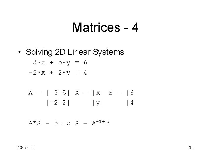
Matrices - 4 • Solving 2 D Linear Systems 3*x + 5*y = 6 -2*x + 2*y = 4 A = | 3 5| X = |x| B = |6| |-2 2| |y| |4| A*X = B so X = A-1*B 12/1/2020 21
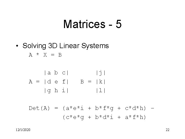
Matrices - 5 • Solving 3 D Linear Systems A * X = B |a b c| A = |d e f| |g h i| |j| B = |k| |l| Det(A) = (a*e*i + b*f*g + c*d*h) – (c*e*g + b*d*i + a*f*h) 12/1/2020 22
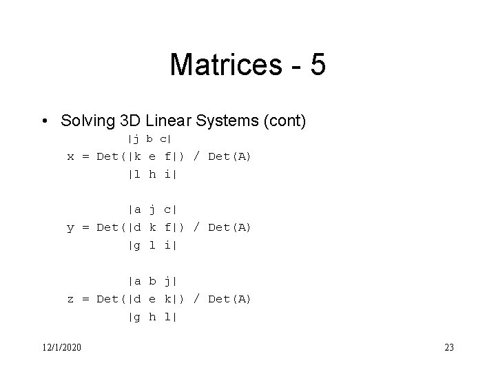
Matrices - 5 • Solving 3 D Linear Systems (cont) |j b c| x = Det(|k e f|) / Det(A) |l h i| |a j c| y = Det(|d k f|) / Det(A) |g l i| |a b j| z = Det(|d e k|) / Det(A) |g h l| 12/1/2020 23
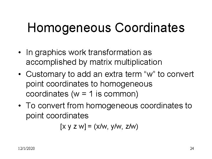
Homogeneous Coordinates • In graphics work transformation as accomplished by matrix multiplication • Customary to add an extra term “w” to convert point coordinates to homogeneous coordinates (w = 1 is common) • To convert from homogeneous coordinates to point coordinates [x y z w] = (x/w, y/w, z/w) 12/1/2020 24
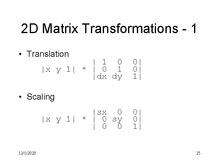
2 D Matrix Transformations - 1 • Translation | 1 0 |x y 1| * | 0 1 |dx dy 0| 0| 1| • Scaling |sx 0 |x y 1| * | 0 sy | 0 0 12/1/2020 0| 0| 1| 25
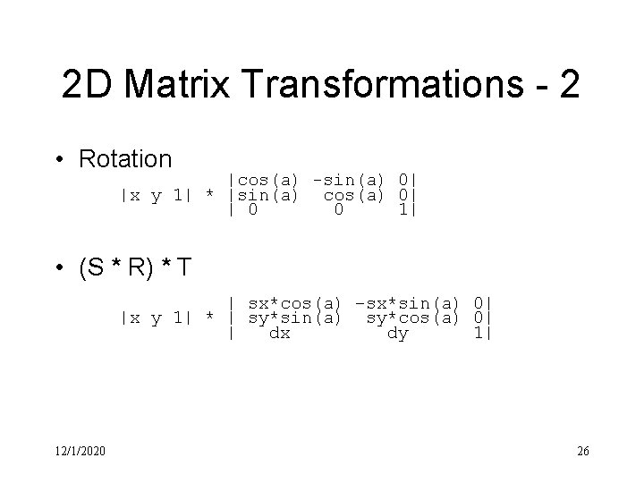
2 D Matrix Transformations - 2 • Rotation |cos(a) -sin(a) 0| |x y 1| * |sin(a) cos(a) 0| | 0 0 1| • (S * R) * T | sx*cos(a) –sx*sin(a) 0| |x y 1| * | sy*sin(a) sy*cos(a) 0| | dx dy 1| 12/1/2020 26
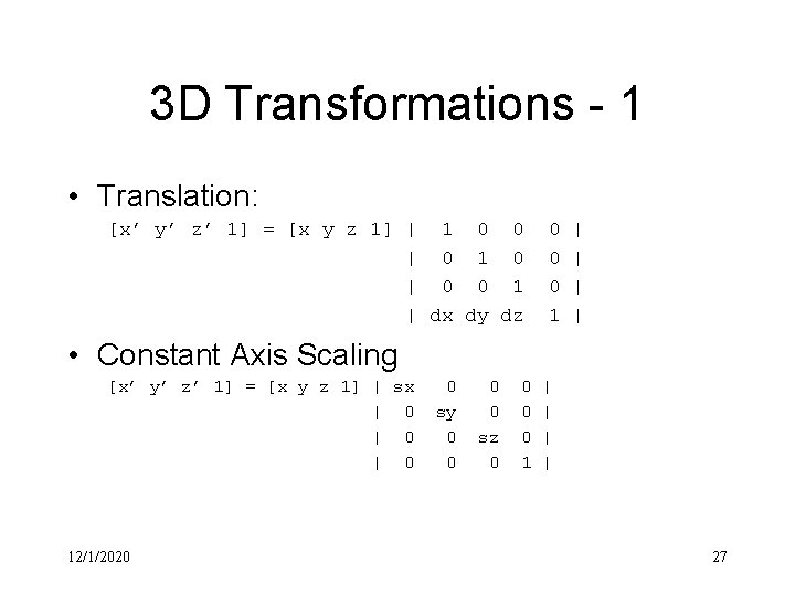
3 D Transformations - 1 • Translation: [x’ y’ z’ 1] = [x y z 1] | 1 0 0 | 0 1 0 | 0 0 1 | dx dy dz 0 0 0 1 | | • Constant Axis Scaling [x’ y’ z’ 1] = [x y z 1] | sx | 0 | 0 12/1/2020 0 sy 0 0 sz 0 0 1 | | 27
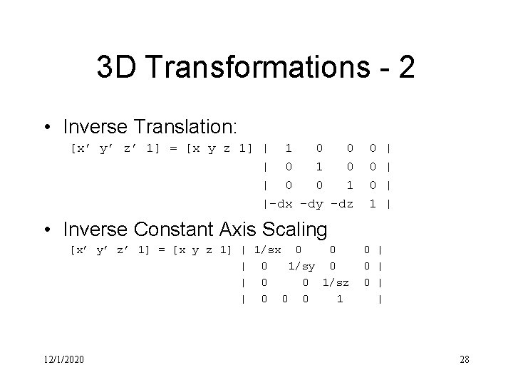
3 D Transformations - 2 • Inverse Translation: [x’ y’ z’ 1] = [x y z 1] | 1 0 0 | 0 1 0 | 0 0 1 |-dx -dy -dz 0 0 0 1 | | • Inverse Constant Axis Scaling [x’ y’ z’ 1] = [x y z 1] | 1/sx 0 0 | 0 1/sy 0 | 0 0 1/sz | 0 0 0 1 12/1/2020 0 | 0 | | 28
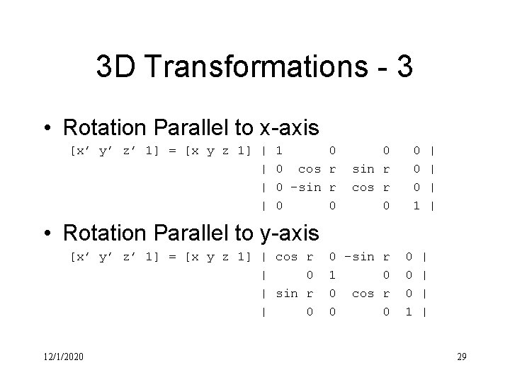
3 D Transformations - 3 • Rotation Parallel to x-axis [x’ y’ z’ 1] = [x y z 1] | | 1 0 0 cos r 0 -sin r 0 0 0 sin r cos r 0 0 1 | | • Rotation Parallel to y-axis [x’ y’ z’ 1] = [x y z 1] | cos r | 0 | sin r | 0 12/1/2020 0 -sin r 1 0 0 cos r 0 0 0 1 | | 29
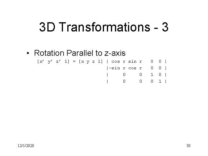
3 D Transformations - 3 • Rotation Parallel to z-axis [x’ y’ z’ 1] = [x y z 1] | cos |-sin | | 12/1/2020 r sin r r cos r 0 0 0 1 | | 30
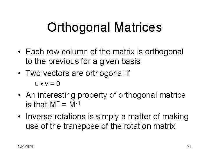
Orthogonal Matrices • Each row column of the matrix is orthogonal to the previous for a given basis • Two vectors are orthogonal if u • v=0 • An interesting property of orthogonal matrics is that MT = M-1 • Inverse rotations is simply a matter of making use of the transpose of the rotation matrix 12/1/2020 31
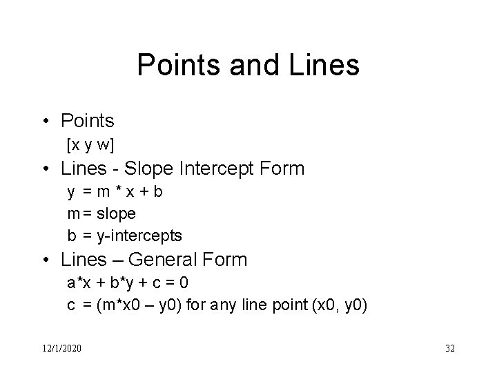
Points and Lines • Points [x y w] • Lines - Slope Intercept Form y =m*x+b m = slope b = y-intercepts • Lines – General Form a*x + b*y + c = 0 c = (m*x 0 – y 0) for any line point (x 0, y 0) 12/1/2020 32

3 D Lines • Consider a line passing through p 0 and p 1 p 0(x 0, y 0, z 0) p 1(x 1, y 1, z 1) v’ = <x 1 -x 0, y 1 -y 0, z 1 -z 0> = <a, b, c> v’ = v / |v| where v = <p 1 – p 0> • Line - Parametric Vector Form p(x, y, z) = p 0 + v’ * t • Line – Explicit Form (x – x 0) / a = (y – y 0) / b = (z – z 0) / c 12/1/2020 33
Figure 4. 38 12/1/2020 34
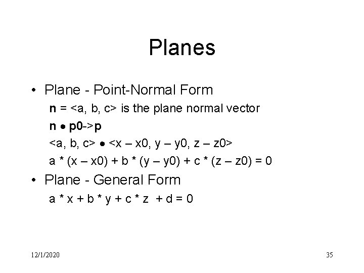
Planes • Plane - Point-Normal Form n = <a, b, c> is the plane normal vector n p 0 ->p <a, b, c> <x – x 0, y – y 0, z – z 0> a * (x – x 0) + b * (y – y 0) + c * (z – z 0) = 0 • Plane - General Form a*x+b*y+c*z +d=0 12/1/2020 35
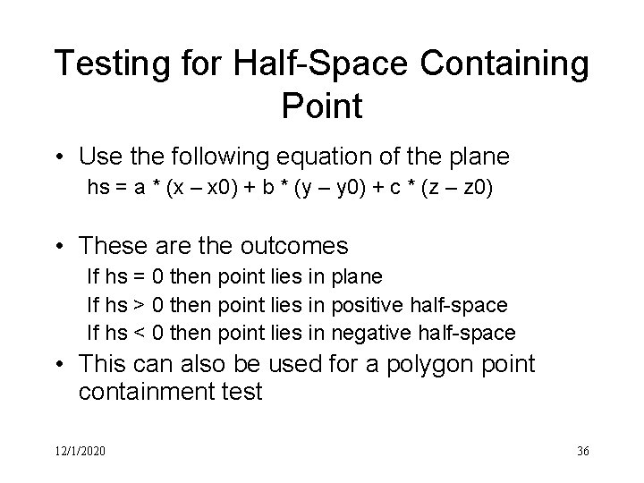
Testing for Half-Space Containing Point • Use the following equation of the plane hs = a * (x – x 0) + b * (y – y 0) + c * (z – z 0) • These are the outcomes If hs = 0 then point lies in plane If hs > 0 then point lies in positive half-space If hs < 0 then point lies in negative half-space • This can also be used for a polygon point containment test 12/1/2020 36
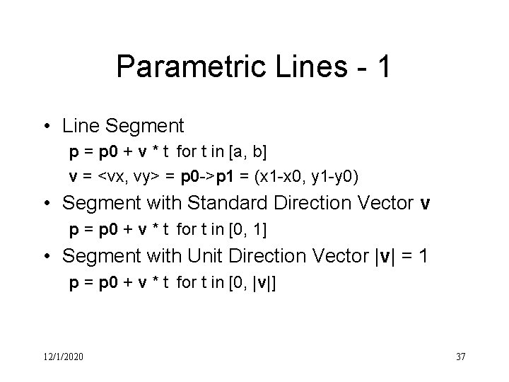
Parametric Lines - 1 • Line Segment p = p 0 + v * t for t in [a, b] v = <vx, vy> = p 0 ->p 1 = (x 1 -x 0, y 1 -y 0) • Segment with Standard Direction Vector v p = p 0 + v * t for t in [0, 1] • Segment with Unit Direction Vector |v| = 1 p = p 0 + v * t for t in [0, |v|] 12/1/2020 37
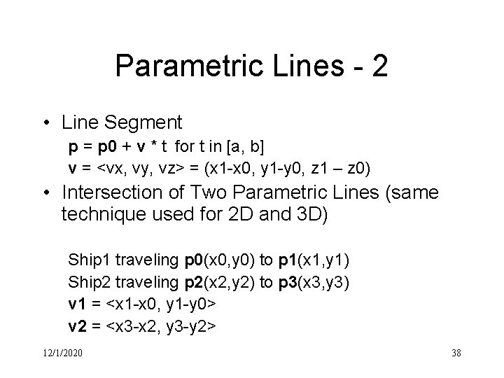
Parametric Lines - 2 • Line Segment p = p 0 + v * t for t in [a, b] v = <vx, vy, vz> = (x 1 -x 0, y 1 -y 0, z 1 – z 0) • Intersection of Two Parametric Lines (same technique used for 2 D and 3 D) Ship 1 traveling p 0(x 0, y 0) to p 1(x 1, y 1) Ship 2 traveling p 2(x 2, y 2) to p 3(x 3, y 3) v 1 = <x 1 -x 0, y 1 -y 0> v 2 = <x 3 -x 2, y 3 -y 2> 12/1/2020 38
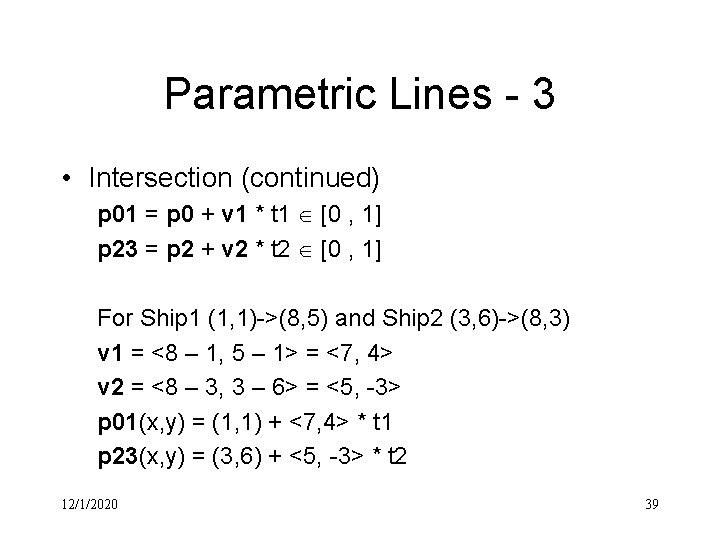
Parametric Lines - 3 • Intersection (continued) p 01 = p 0 + v 1 * t 1 [0 , 1] p 23 = p 2 + v 2 * t 2 [0 , 1] For Ship 1 (1, 1)->(8, 5) and Ship 2 (3, 6)->(8, 3) v 1 = <8 – 1, 5 – 1> = <7, 4> v 2 = <8 – 3, 3 – 6> = <5, -3> p 01(x, y) = (1, 1) + <7, 4> * t 1 p 23(x, y) = (3, 6) + <5, -3> * t 2 12/1/2020 39
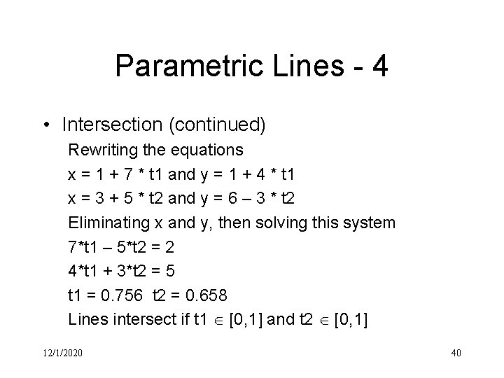
Parametric Lines - 4 • Intersection (continued) Rewriting the equations x = 1 + 7 * t 1 and y = 1 + 4 * t 1 x = 3 + 5 * t 2 and y = 6 – 3 * t 2 Eliminating x and y, then solving this system 7*t 1 – 5*t 2 = 2 4*t 1 + 3*t 2 = 5 t 1 = 0. 756 t 2 = 0. 658 Lines intersect if t 1 [0, 1] and t 2 [0, 1] 12/1/2020 40
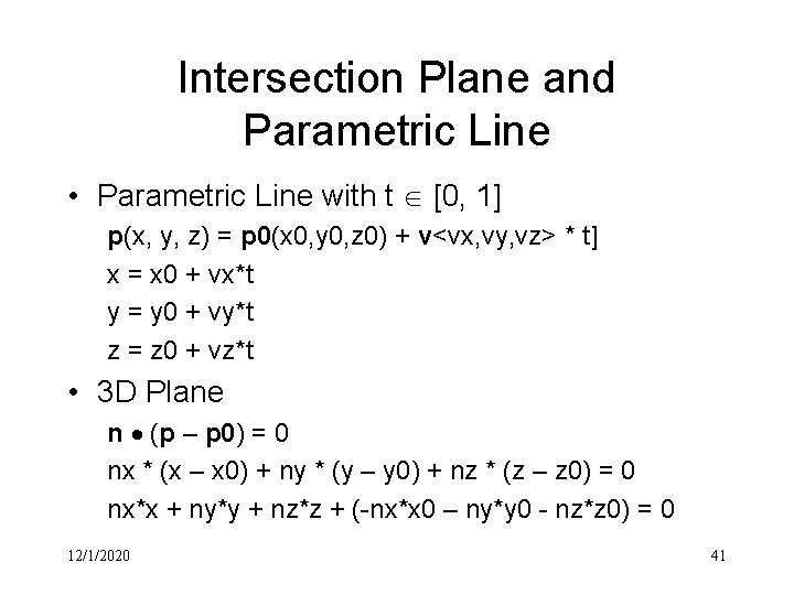
Intersection Plane and Parametric Line • Parametric Line with t [0, 1] p(x, y, z) = p 0(x 0, y 0, z 0) + v<vx, vy, vz> * t] x = x 0 + vx*t y = y 0 + vy*t z = z 0 + vz*t • 3 D Plane n (p – p 0) = 0 nx * (x – x 0) + ny * (y – y 0) + nz * (z – z 0) = 0 nx*x + ny*y + nz*z + (-nx*x 0 – ny*y 0 - nz*z 0) = 0 12/1/2020 41
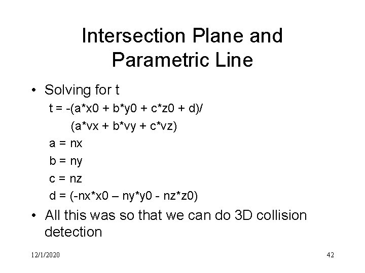
Intersection Plane and Parametric Line • Solving for t t = -(a*x 0 + b*y 0 + c*z 0 + d)/ (a*vx + b*vy + c*vz) a = nx b = ny c = nz d = (-nx*x 0 – ny*y 0 - nz*z 0) • All this was so that we can do 3 D collision detection 12/1/2020 42
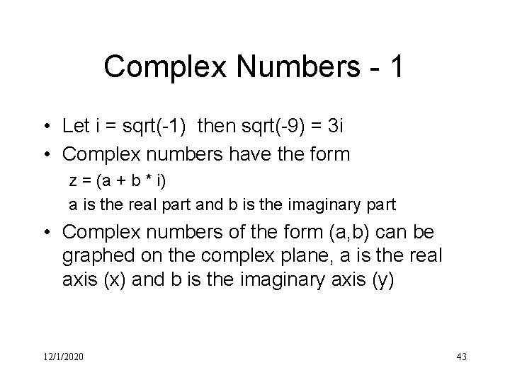
Complex Numbers - 1 • Let i = sqrt(-1) then sqrt(-9) = 3 i • Complex numbers have the form z = (a + b * i) a is the real part and b is the imaginary part • Complex numbers of the form (a, b) can be graphed on the complex plane, a is the real axis (x) and b is the imaginary axis (y) 12/1/2020 43
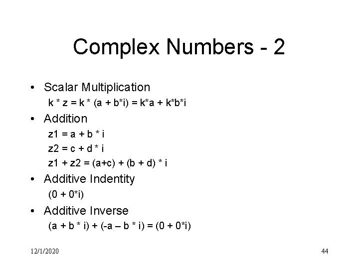
Complex Numbers - 2 • Scalar Multiplication k * z = k * (a + b*i) = k*a + k*b*i • Addition z 1 = a + b * i z 2 = c + d * i z 1 + z 2 = (a+c) + (b + d) * i • Additive Indentity (0 + 0*i) • Additive Inverse (a + b * i) + (-a – b * i) = (0 + 0*i) 12/1/2020 44
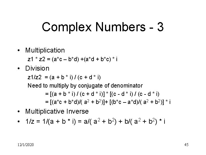
Complex Numbers - 3 • Multiplication z 1 * z 2 = (a*c – b*d) +(a*d + b*c) * i • Division z 1/z 2 = (a + b * i) / (c + d * i) Need to multiply by conjugate of denominator = [(a + b * i) / (c + d * i)] * [(c - d * i) / (c - d * i) = [(a*c + b*d)/( a 2 + b 2)]+ [(b*c – a*d)/( a 2 + b 2)] * i • Multiplicative Inverse • 1/z = 1/(a + b * i) = a/( a 2 + b 2) + b/( a 2 + b 2) * i 12/1/2020 45
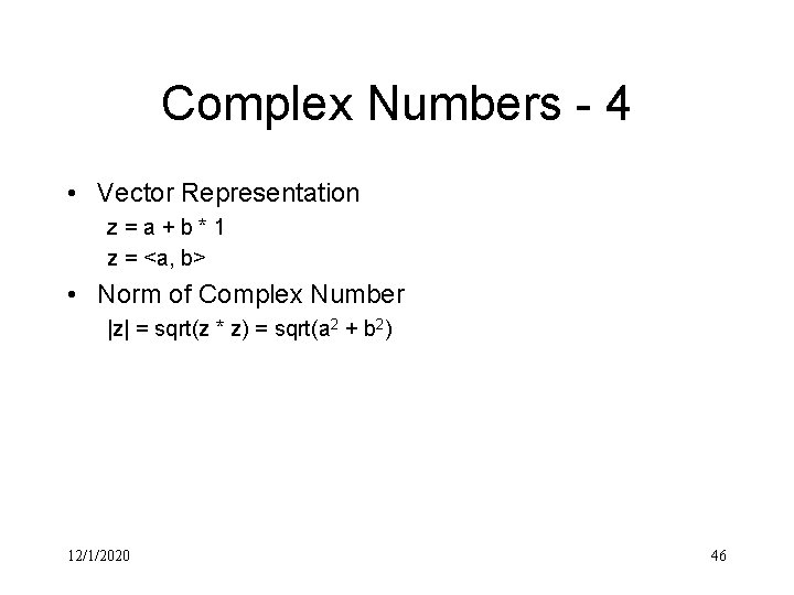
Complex Numbers - 4 • Vector Representation z=a+b*1 z = <a, b> • Norm of Complex Number |z| = sqrt(z * z) = sqrt(a 2 + b 2) 12/1/2020 46
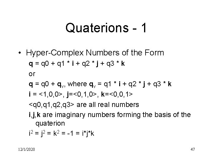
Quaterions - 1 • Hyper-Complex Numbers of the Form q = q 0 + q 1 * i + q 2 * j + q 3 * k or q = q 0 + qv, where qv = q 1 * i + q 2 * j + q 3 * k i = <1, 0, 0>, j=<0, 1, 0>, k=<0, 0, 1> <q 0, q 1, q 2, q 3> are all real numbers i, j, k are imaginary numbers forming the basis of the quaterion i 2 = j 2 = k 2 = -1 = i*j*k 12/1/2020 47
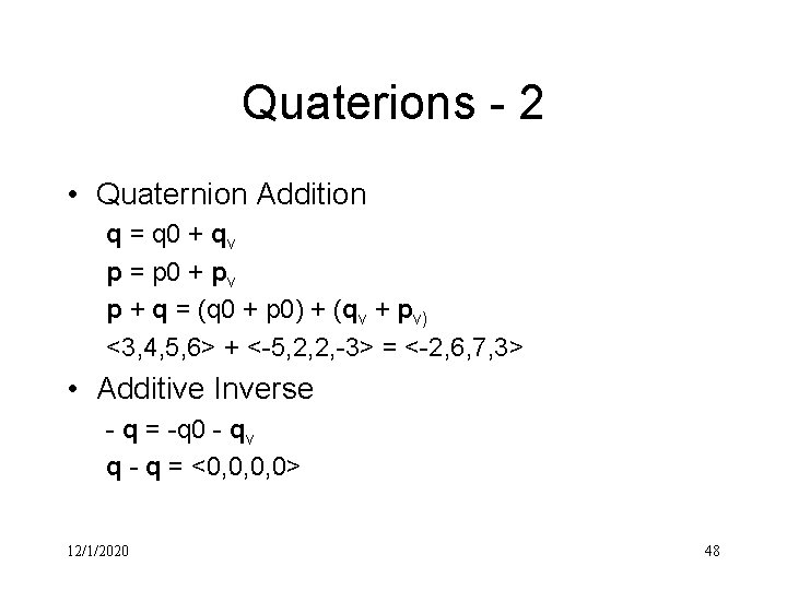
Quaterions - 2 • Quaternion Addition q = q 0 + qv p = p 0 + pv p + q = (q 0 + p 0) + (qv + pv) <3, 4, 5, 6> + <-5, 2, 2, -3> = <-2, 6, 7, 3> • Additive Inverse - q = -q 0 - qv q - q = <0, 0, 0, 0> 12/1/2020 48
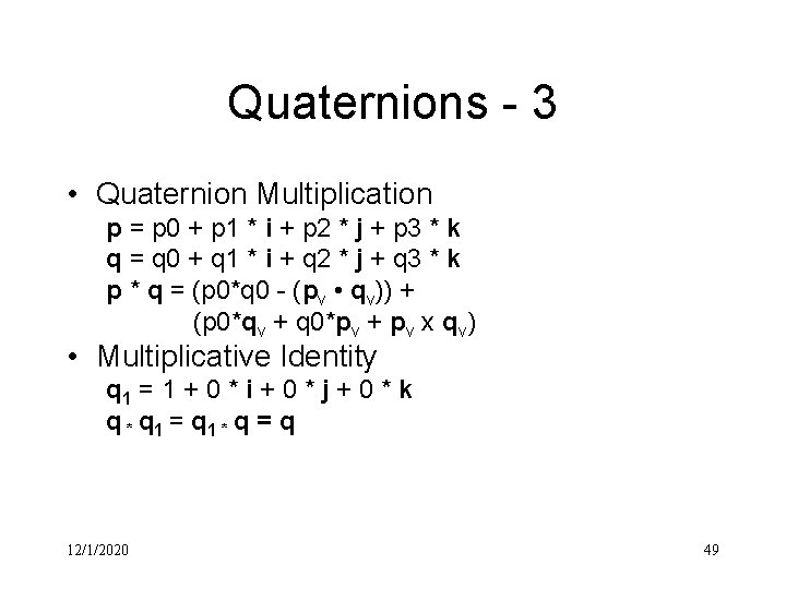
Quaternions - 3 • Quaternion Multiplication p = p 0 + p 1 * i + p 2 * j + p 3 * k q = q 0 + q 1 * i + q 2 * j + q 3 * k p * q = (p 0*q 0 - (pv • qv)) + (p 0*qv + q 0*pv + pv x qv) • Multiplicative Identity q 1 = 1 + 0 * i + 0 * j + 0 * k q * q 1 = q 1 * q = q 12/1/2020 49
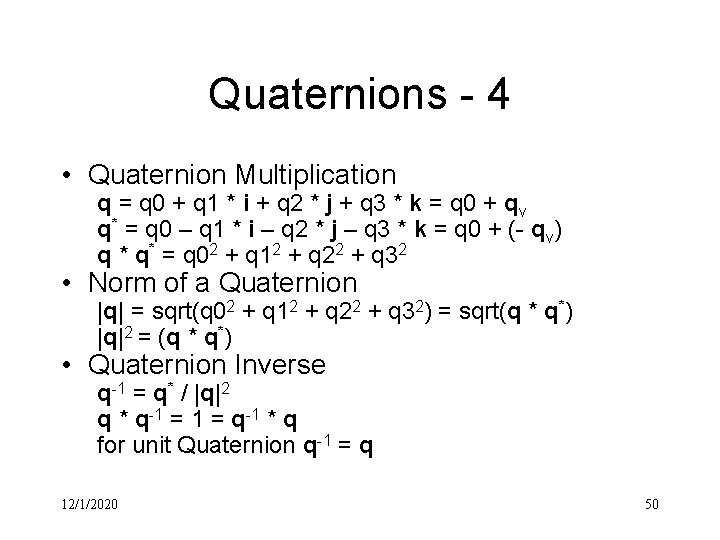
Quaternions - 4 • Quaternion Multiplication q = q 0 + q 1 * i + q 2 * j + q 3 * k = q 0 + qv q* = q 0 – q 1 * i – q 2 * j – q 3 * k = q 0 + (- qv) q * q* = q 02 + q 12 + q 22 + q 32 • Norm of a Quaternion |q| = sqrt(q 02 + q 12 + q 22 + q 32) = sqrt(q * q*) |q|2 = (q * q*) • Quaternion Inverse q-1 = q* / |q|2 q * q-1 = q-1 * q for unit Quaternion q-1 = q 12/1/2020 50
Quaternion Uses • Can be for ordinary 3 D rotatiosn and interpolation of rotation • La. Mothe uses quaternions to interpolate between different camera angles • Quaternions with their 4 D character can handle rotation of a 3 D object around an arbitrary axis more easily than vectors • So if you have lots of matrix multiplication in a loop switch to quaternions 12/1/2020 51

Figure 4. 44 12/1/2020 52
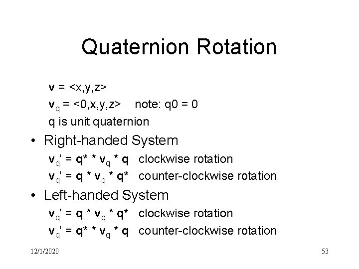
Quaternion Rotation v = <x, y, z> vq = <0, x, y, z> note: q 0 = 0 q is unit quaternion • Right-handed System vq’ = q* * vq * q clockwise rotation vq’ = q * vq * q* counter-clockwise rotation • Left-handed System vq’ = q * vq * q* clockwise rotation vq’ = q* * vq * q counter-clockwise rotation 12/1/2020 53

Figure 4. 45 12/1/2020 54
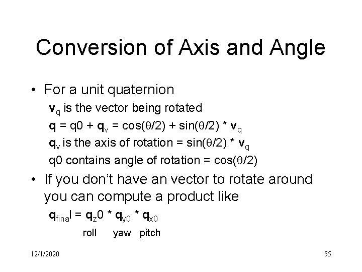
Conversion of Axis and Angle • For a unit quaternion vq is the vector being rotated q = q 0 + qv = cos( /2) + sin( /2) * vq qv is the axis of rotation = sin( /2) * vq q 0 contains angle of rotation = cos( /2) • If you don’t have an vector to rotate around you can compute a product like qfinal = qz 0 * qy 0 * qx 0 roll 12/1/2020 yaw pitch 55

Euler Angles for Quaternion - 1 qx 0 = cos(x 0 / 2) + sin(x 0 / 2) * i + 0 * j + 0 * k q 0 = cos(x 0 / 2) , qv = <sin(x 0 / 2) , 0, 0> qy 0 = cos(y 0 / 2) + 0 * i + sin(y 0 / 2 * j + 0 * k q 0 = cos(y 0 / 2) , qv = <0, sin(y 0 / 2) , 0> qz 0 = cos(z 0 / 2) + 0 * i + 0 * j + sin(z 0 / 2) * k q 0 = cos(z 0 / 2) , qv = <0, 0, sin(z 0 / 2)> • Rotation vq’(0, x’, y’, z’) = (qz 0 * qy 0 * qx 0) * vq * (qz 0 * qy 0 * qx 0)* vq = <0, y, y, z> 12/1/2020 56
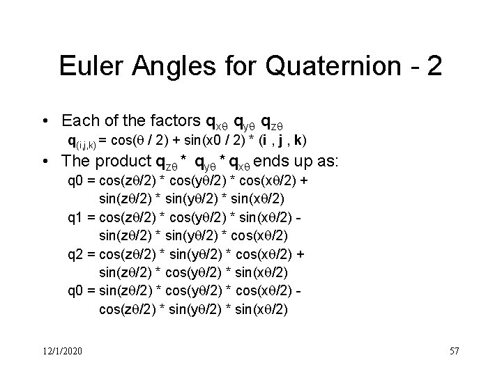
Euler Angles for Quaternion - 2 • Each of the factors qx qy qz q(i, j, k) = cos( / 2) + sin(x 0 / 2) * (i , j , k) • The product qz * qy * qx ends up as: q 0 = cos(z /2) * cos(y /2) * cos(x /2) + sin(z /2) * sin(y /2) * sin(x /2) q 1 = cos(z /2) * cos(y /2) * sin(x /2) sin(z /2) * sin(y /2) * cos(x /2) q 2 = cos(z /2) * sin(y /2) * cos(x /2) + sin(z /2) * cos(y /2) * sin(x /2) q 0 = sin(z /2) * cos(y /2) * cos(x /2) cos(z /2) * sin(y /2) * sin(x /2) 12/1/2020 57

Calculus Rdeview • Pages 337 to 361 12/1/2020 58
- Slides: 58