3 D Computer Vision CSc 83020 Clustering methods

3 -D Computer Vision CSc 83020 Clustering methods and boundary representations 3 -D Computer Vision CSc 83020 – Ioannis Stamos

Image Segmentation n n Generate clusters (regions) of pixels that correspond to meaningful entities. Use metrics of “closeness” between values. Use algorithms for combining “close” values. Apply other constraints (connectivity). 3 -D Computer Vision CSc 83020 – Ioannis Stamos

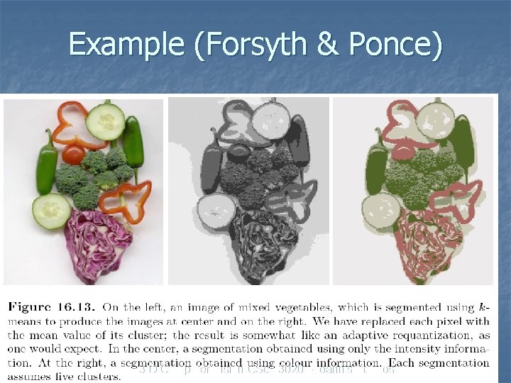
Example (Forsyth & Ponce) 3 -D Computer Vision CSc 83020 – Ioannis Stamos

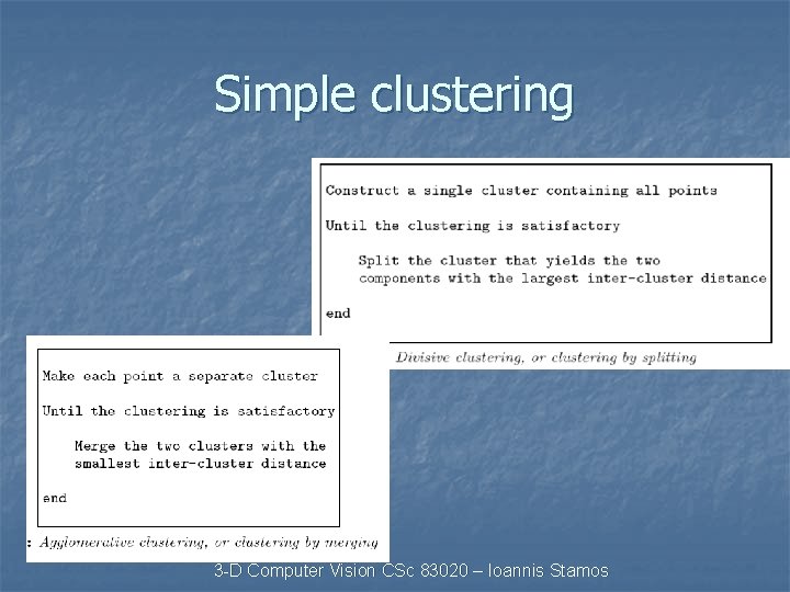
Simple Clustering Methods n Divisive clustering Everything is a big cluster at beginning n Split recursively n n Agglomerative clustering Each data (pixel) is a cluster n Merge n 3 -D Computer Vision CSc 83020 – Ioannis Stamos

Simple clustering 3 -D Computer Vision CSc 83020 – Ioannis Stamos

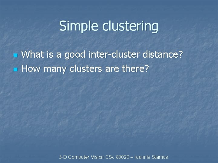
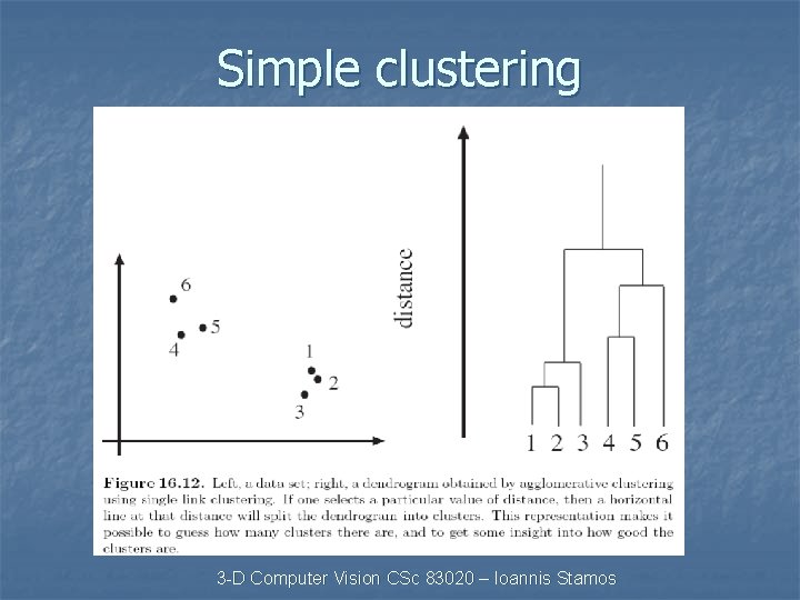
Simple clustering n n What is a good inter-cluster distance? How many clusters are there? 3 -D Computer Vision CSc 83020 – Ioannis Stamos

Simple clustering 3 -D Computer Vision CSc 83020 – Ioannis Stamos

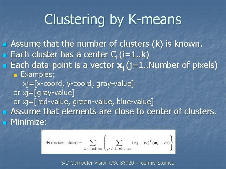
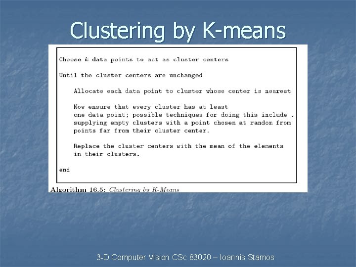
Clustering by K-means n n n Assume that the number of clusters (k) is known. Each cluster has a center Ci (i=1. . k) Each data-point is a vector xj (j=1. . Number of pixels) Examples: xj=[x-coord, y-coord, gray-value] or xj=[red-value, green-value, blue-value] n n n Assume that elements are close to center of clusters. Minimize: 3 -D Computer Vision CSc 83020 – Ioannis Stamos

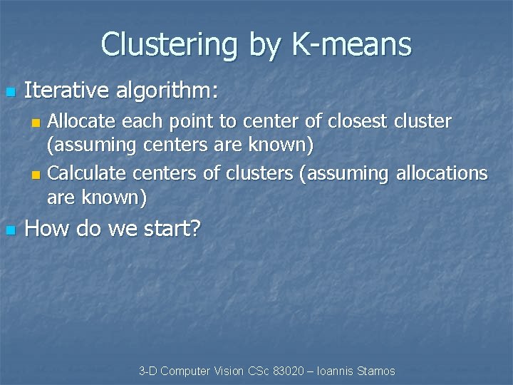
Clustering by K-means n Iterative algorithm: Allocate each point to center of closest cluster (assuming centers are known) n Calculate centers of clusters (assuming allocations are known) n n How do we start? 3 -D Computer Vision CSc 83020 – Ioannis Stamos

Clustering by K-means 3 -D Computer Vision CSc 83020 – Ioannis Stamos

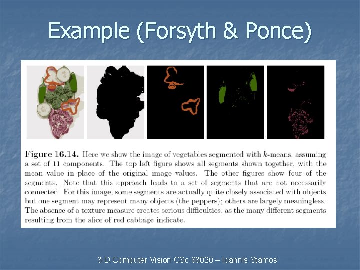
Example (Forsyth & Ponce) 3 -D Computer Vision CSc 83020 – Ioannis Stamos

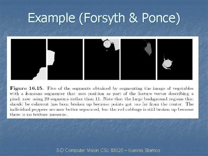
Example (Forsyth & Ponce) 3 -D Computer Vision CSc 83020 – Ioannis Stamos

Example (Forsyth & Ponce) 3 -D Computer Vision CSc 83020 – Ioannis Stamos

RANSAC n n n RANdom SAmple Consensus Model fitting method Line-fitting example Fitting a line to a set of edges with 50% outliers n Least squares would fail n Solution: M-estimator or RANSAC n 3 -D Computer Vision CSc 83020 – Ioannis Stamos

RANSAC (line-fitting example) n n Two edges (wout normal) define a line. General idea: n n n Pick two points. Write the equation of the line. Check how many other points are “close” to line. If number of “close” points is above threshold, done Otherwise, pick two new points. Questions: n n Which points to pick? Complexity in worst case? 3 -D Computer Vision CSc 83020 – Ioannis Stamos

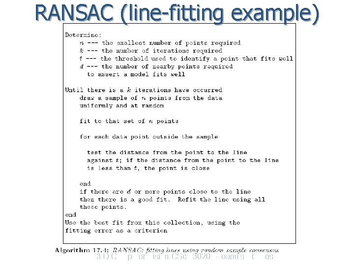
RANSAC (line-fitting example) 3 -D Computer Vision CSc 83020 – Ioannis Stamos

RANSAC (line-fitting example) How large should k (max. number of iterations) be? 3 -D Computer Vision CSc 83020 – Ioannis Stamos

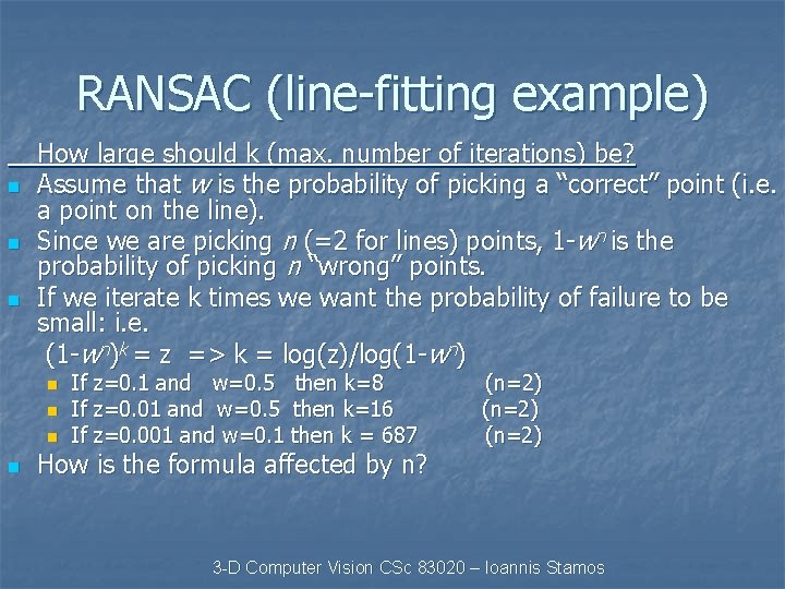
RANSAC (line-fitting example) n n n How large should k (max. number of iterations) be? Assume that w is the probability of picking a “correct” point (i. e. a point on the line). Since we are picking n (=2 for lines) points, 1 -wn is the probability of picking n “wrong” points. If we iterate k times we want the probability of failure to be small: i. e. (1 -wn)k = z => k = log(z)/log(1 -wn) n n If z=0. 1 and w=0. 5 then k=8 If z=0. 01 and w=0. 5 then k=16 If z=0. 001 and w=0. 1 then k = 687 How is the formula affected by n? (n=2) 3 -D Computer Vision CSc 83020 – Ioannis Stamos

RANSAC (Conclusions) n n When can this method be successful? Can we detect circles? n n In that case how many points do you need to fit a circle? Can we detect other shapes? 3 -D Computer Vision CSc 83020 – Ioannis Stamos

Boundary representation of regions 3 -D Computer Vision CSc 83020 – Ioannis Stamos

Representation of 2 -D Geometric Structures To MATCH image boundary/region with MODEL boundary/region, they must represented in the same manner. • Boundary Representation • Snakes – Extraction of arbitrary contours from image. • Region Representation 3 -D Computer Vision CSc 83020 – Ioannis Stamos

Representation Issues n n Compact: Easy to Store & Match. Easy to manipulate & compute properties. Captures Object/Model shape. Computationally efficient. 3 -D Computer Vision CSc 83020 – Ioannis Stamos

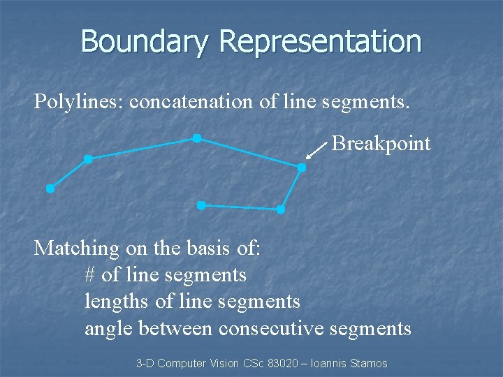
Boundary Representation Polylines: concatenation of line segments. Breakpoint Matching on the basis of: # of line segments lengths of line segments angle between consecutive segments 3 -D Computer Vision CSc 83020 – Ioannis Stamos

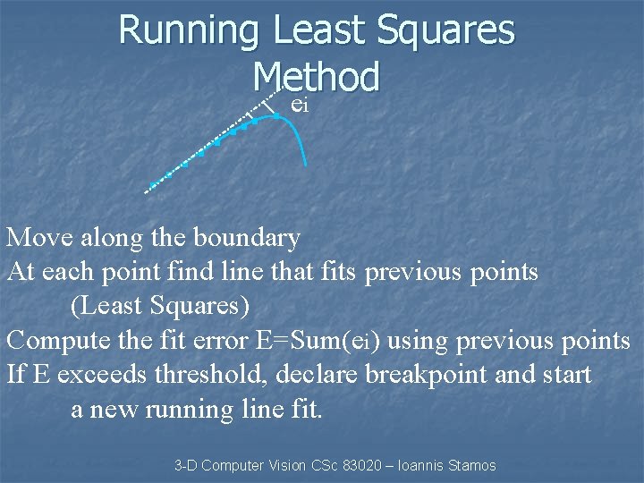
Running Least Squares Method ei Move along the boundary At each point find line that fits previous points (Least Squares) Compute the fit error E=Sum(ei) using previous points If E exceeds threshold, declare breakpoint and start a new running line fit. 3 -D Computer Vision CSc 83020 – Ioannis Stamos

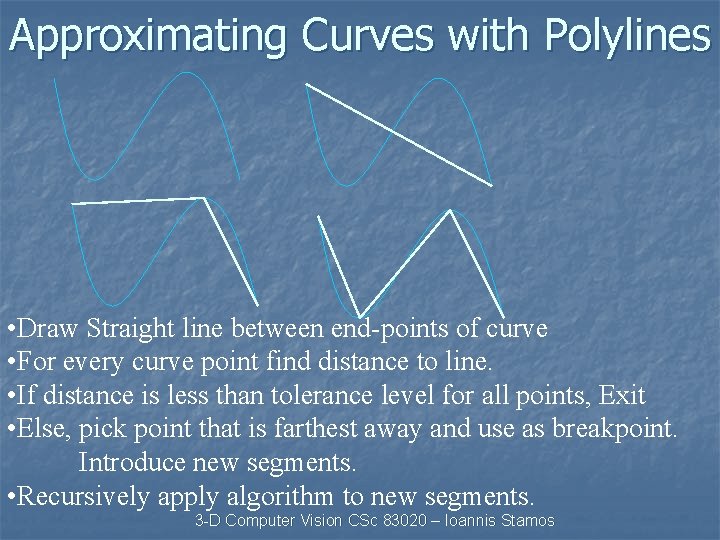
Approximating Curves with Polylines • Draw Straight line between end-points of curve • For every curve point find distance to line. • If distance is less than tolerance level for all points, Exit • Else, pick point that is farthest away and use as breakpoint. Introduce new segments. • Recursively apply algorithm to new segments. 3 -D Computer Vision CSc 83020 – Ioannis Stamos

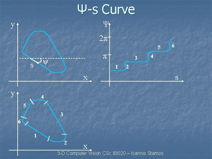
Ψ-s Curve y Ψ 2π 5 π ψ s 3 1 4 2 x y 4 5 3 6 1 2 6 x 3 -D Computer Vision CSc 83020 – Ioannis Stamos s

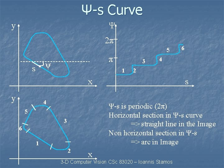
Ψ-s Curve y Ψ 2π 5 π ψ s 3 1 4 2 x y 4 6 s Ψ-s is periodic (2π) Horizontal section in Ψ-s curve => straight line in the Image Non horizontal section in Ψ-s => arc in Image 5 3 6 1 2 x 3 -D Computer Vision CSc 83020 – Ioannis Stamos

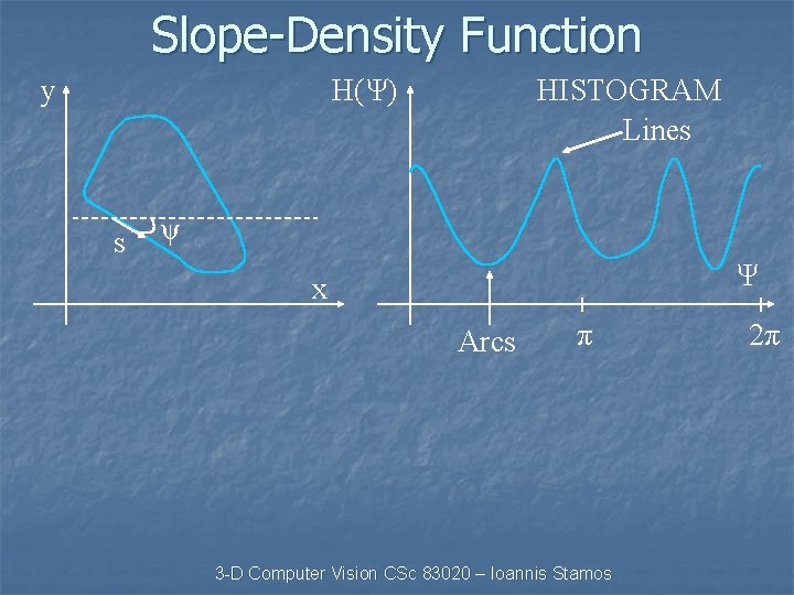
Slope-Density Function y H(Ψ) s HISTOGRAM Lines ψ Ψ x Arcs π 3 -D Computer Vision CSc 83020 – Ioannis Stamos 2π

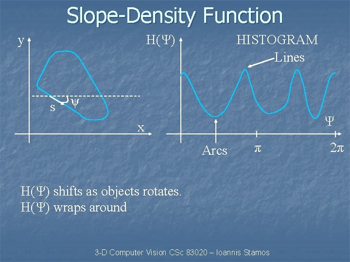
Slope-Density Function y H(Ψ) s HISTOGRAM Lines ψ Ψ x Arcs π H(Ψ) shifts as objects rotates. H(Ψ) wraps around 3 -D Computer Vision CSc 83020 – Ioannis Stamos 2π

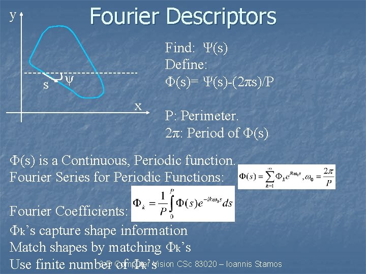
Fourier Descriptors y s Find: Ψ(s) Define: Φ(s)= Ψ(s)-(2πs)/P ψ x P: Perimeter. 2π: Period of Φ(s) is a Continuous, Periodic function. Fourier Series for Periodic Functions: Fourier Coefficients: Φk’s capture shape information Match shapes by matching Φk’s 3 -D Computer Use finite number of Φk’s. Vision CSc 83020 – Ioannis Stamos

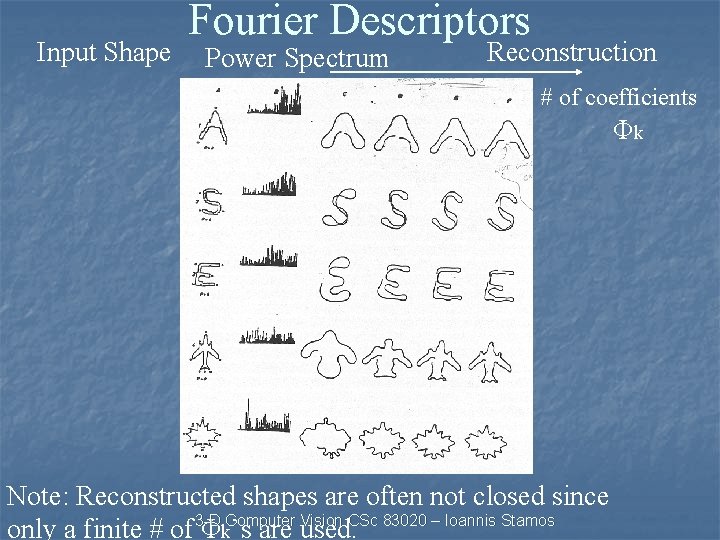
Input Shape Fourier Descriptors Power Spectrum Reconstruction # of coefficients Φk Note: Reconstructed shapes are often not closed since Vision CSc 83020 – Ioannis Stamos only a finite # of 3 -D Φk. Computer ’s are used.

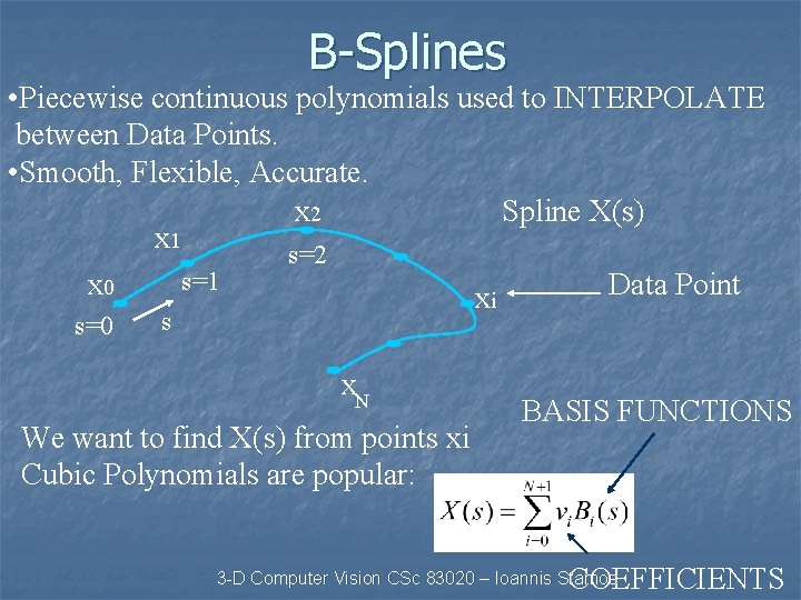
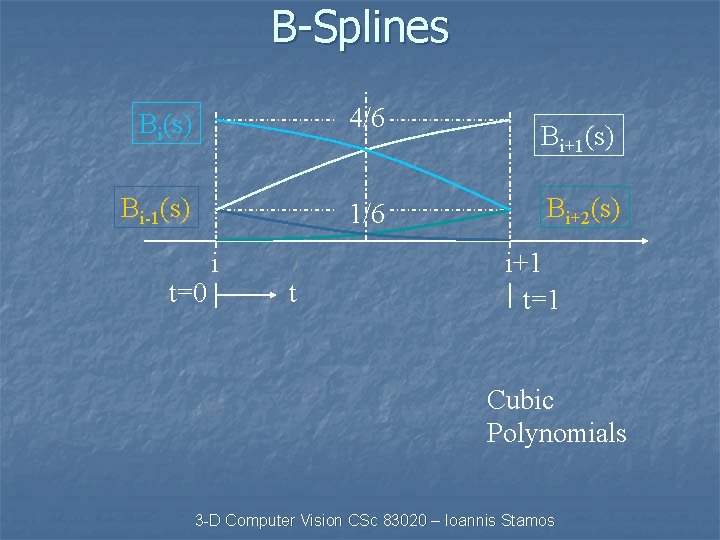
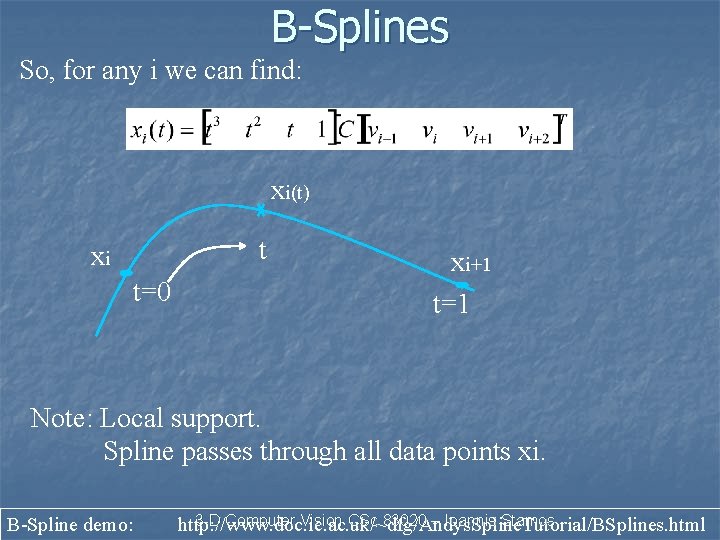
B-Splines • Piecewise continuous polynomials used to INTERPOLATE between Data Points. • Smooth, Flexible, Accurate. x 2 Spline X(s) x 1 s=2 s=1 x 0 Data Point xi s=0 s x. N We want to find X(s) from points xi Cubic Polynomials are popular: BASIS FUNCTIONS COEFFICIENTS 3 -D Computer Vision CSc 83020 – Ioannis Stamos

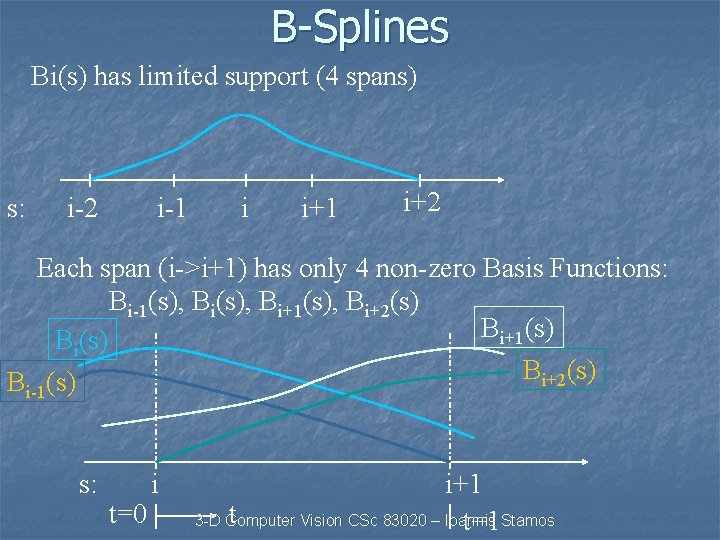
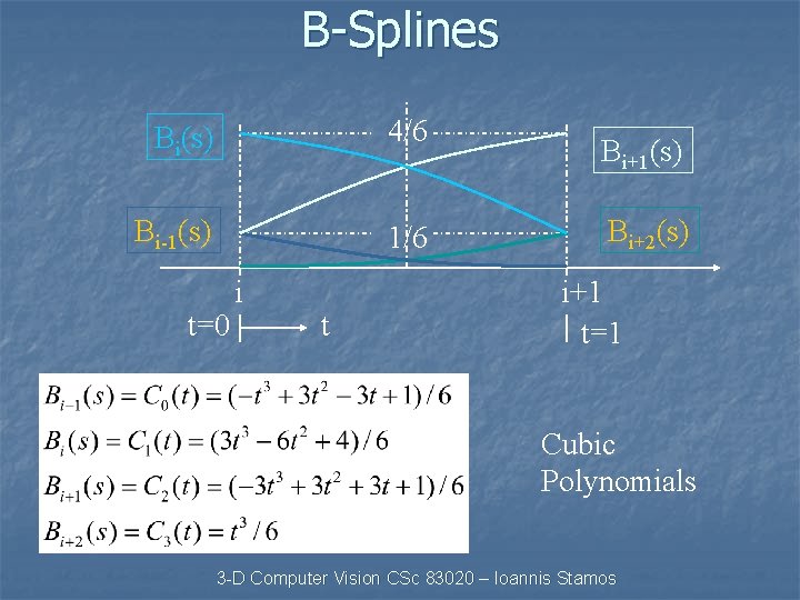
B-Splines Bi(s) has limited support (4 spans) s: i-2 i-1 i i+1 i+2 Each span (i->i+1) has only 4 non-zero Basis Functions: Bi-1(s), Bi+1(s), Bi+2(s) Bi+1(s) Bi+2(s) Bi-1(s) s: t=0 i i+1 t 3 -D Computer Vision CSc 83020 – Ioannis t=1 Stamos

B-Splines Bi(s) 4/6 Bi-1(s) 1/6 t=0 i t Bi+1(s) Bi+2(s) i+1 t=1 Cubic Polynomials 3 -D Computer Vision CSc 83020 – Ioannis Stamos

B-Splines Bi(s) 4/6 Bi-1(s) 1/6 t=0 i t Bi+1(s) Bi+2(s) i+1 t=1 Cubic Polynomials 3 -D Computer Vision CSc 83020 – Ioannis Stamos

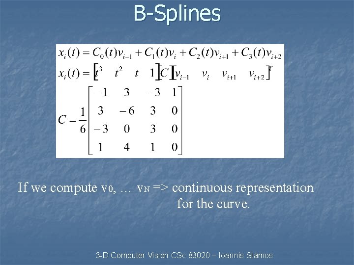
B-Splines If we compute v 0, … v. N => continuous representation for the curve. 3 -D Computer Vision CSc 83020 – Ioannis Stamos

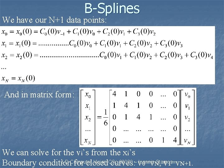
B-Splines We have our N+1 data points: And in matrix form: We can solve for the vi’s from the xi’s 3 -D Computer Vision CSc 83020 – v Ioannis Stamos Boundary condition for closed curves: 0=v. N , v 1=v. N+1.

B-Splines So, for any i we can find: xi(t) t xi t=0 xi+1 t=1 Note: Local support. Spline passes through all data points xi. B-Spline demo: 3 -D Computer Vision CSc 83020 – Ioannis Stamos http: //www. doc. ic. ac. uk/~dfg/Andys. Spline. Tutorial/BSplines. html

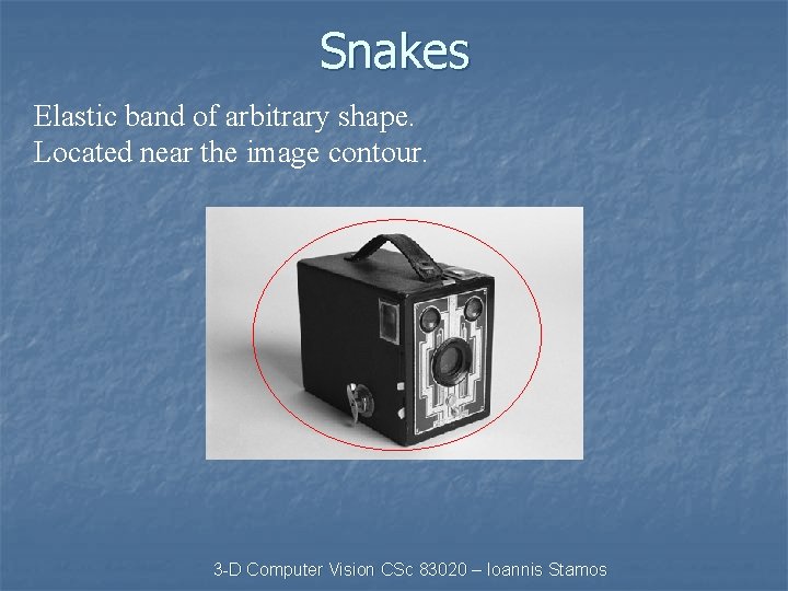
Snakes Elastic band of arbitrary shape. Located near the image contour. 3 -D Computer Vision CSc 83020 – Ioannis Stamos

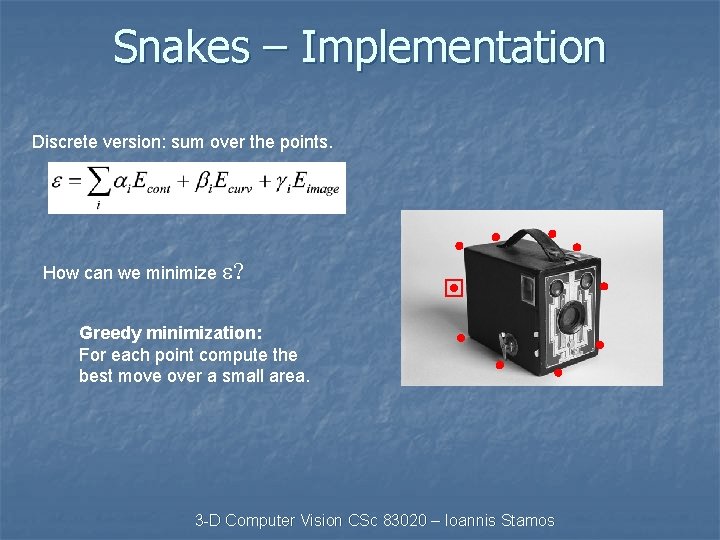
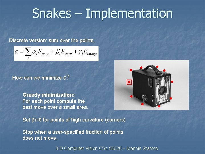
Snakes – Implementation Discrete version: sum over the points. How can we minimize e? Greedy minimization: For each point compute the best move over a small area. 3 -D Computer Vision CSc 83020 – Ioannis Stamos

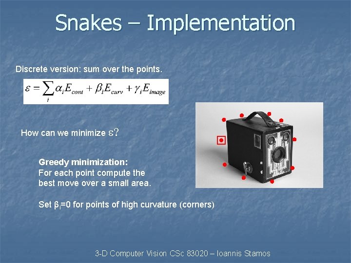
Snakes – Implementation Discrete version: sum over the points. How can we minimize e? Greedy minimization: For each point compute the best move over a small area. Set βi=0 for points of high curvature (corners) 3 -D Computer Vision CSc 83020 – Ioannis Stamos

Snakes – Implementation Discrete version: sum over the points. How can we minimize e? Greedy minimization: For each point compute the best move over a small area. Set βi=0 for points of high curvature (corners) Stop when a user-specified fraction of points does not move. 3 -D Computer Vision CSc 83020 – Ioannis Stamos

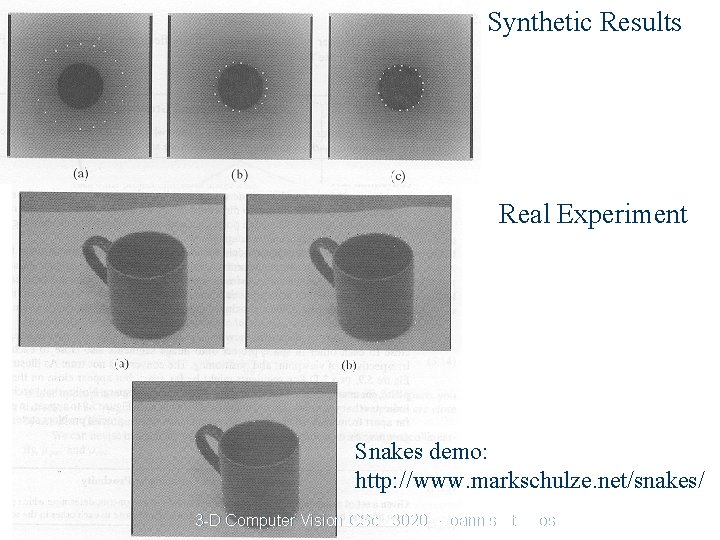
Synthetic Results Real Experiment Snakes demo: http: //www. markschulze. net/snakes/ 3 -D Computer Vision CSc 83020 – Ioannis Stamos

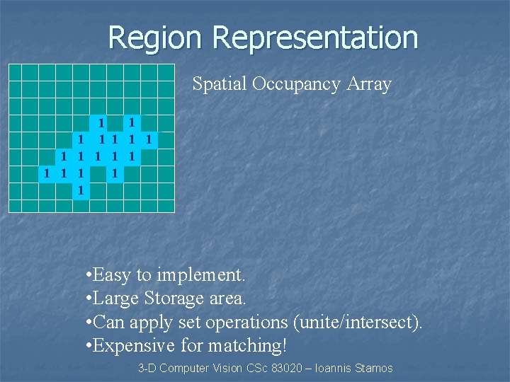
Region Representation Spatial Occupancy Array 1 1 1 1 1 • Easy to implement. • Large Storage area. • Can apply set operations (unite/intersect). • Expensive for matching! 3 -D Computer Vision CSc 83020 – Ioannis Stamos

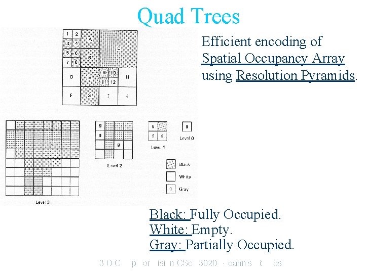
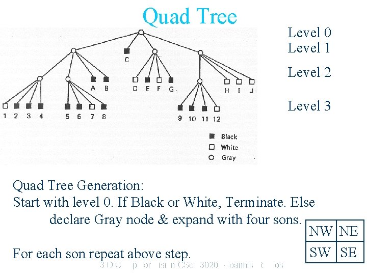
Quad Trees Efficient encoding of Spatial Occupancy Array using Resolution Pyramids. Black: Fully Occupied. White: Empty. Gray: Partially Occupied. 3 -D Computer Vision CSc 83020 – Ioannis Stamos

Quad Tree Level 0 Level 1 Level 2 Level 3 Quad Tree Generation: Start with level 0. If Black or White, Terminate. Else declare Gray node & expand with four sons. NW NE SW SE For each son repeat above step. 3 -D Computer Vision CSc 83020 – Ioannis Stamos