3 D Computer Vision and Video Computing Image

3 D Computer Vision and Video Computing Image Formation CSc 80000 Section 2 Spring 2005 Lecture 2 – Part 2 Image Formation http: //www-cs. engr. ccny. cuny. edu/~zhu/GC-Spring 2005/CSc 80000 -2 -Vision. Course. html

3 D Computer Vision and Video Computing Acknowledgements The slides in this lecture were adopted from Professor Allen Hanson University of Massachusetts at Amherst

3 D Computer Vision and Video Computing n Light and Optics l l l n n Lecture Outline Pinhole camera model Perspective projection Thin lens model Fundamental equation Distortion: spherical & chromatic aberration, radial distortion (*optional) Reflection and Illumination: color, lambertian and specular surfaces, Phong, BDRF (*optional) Sensing Light Conversion to Digital Images Sampling Theorem Other Sensors: frequency, type, ….

3 D Computer Vision Abstract Image and Video Computing n n n An image can be represented by an image function whose general form is f(x, y) is a vector-valued function whose arguments represent a pixel location. The value of f(x, y) can have different interpretations in different kinds of images. Examples Intensity Image Range Image Color Image Video - f(x, y) = intensity of the scene - f(x, y) = depth of the scene from imaging system - f(x, y) = {fr(x, y), fg(x, y), fb(x, y)} - f(x, y, t) = temporal image sequence

3 D Computer Vision and Video Computing n Basic Radiometry is the part of image formation concerned with the relation among the amounts of light energy emitted from light sources, reflected from surfaces, and registered by sensors.

3 D Computer Vision and Video Computing n Light and Matter The interaction between light and matter can take many forms: l l l Reflection Refraction Diffraction Absorption Scattering

3 D Computer Vision and Video Computing n Typical imaging scenario: l l n Lecture Assumptions visible light ideal lenses standard sensor (e. g. TV camera) opaque objects Goal To create 'digital' images which can be processed to recover some of the characteristics of the 3 D world which was imaged.

3 D Computer Vision and Video Computing Steps World Optics Sensor Signal Digitizer Digital Representation World Optics Sensor Signal Digitizer Digital Rep. reality focus {light} from world on sensor converts {light} to {electrical energy} representation of incident light as continuous electrical energy converts continuous signal to discrete signal final representation of reality in computer memory

3 D Computer Vision and Video Computing n Geometry l n concerned with the relationship between the amount of light radiating from a surface and the amount incident at its image Photometry l n concerned with the relationship between points in the three-dimensional world and their images Radiometry l n Factors in Image Formation concerned with ways of measuring the intensity of light Digitization l concerned with ways of converting continuous signals (in both space and time) to digital approximations

3 D Computer Vision and Video Computing Image Formation

3 D Computer Vision Geometry and Video Computing n Geometry describes the projection of: three-dimensional (3 D) world n n two-dimensional (2 D) image plane. Typical Assumptions l Light travels in a straight line Optical Axis: the axis perpendicular to the image plane and passing through the pinhole (also called the central projection ray) Each point in the image corresponds to a particular direction defined by a ray from that point through the pinhole. Various kinds of projections: l - perspective - oblique l - orthographic - isometric l - spherical

3 D Computer Vision and Video Computing n Two models are commonly used: l l n Pin-hole camera Optical system composed of lenses Pin-hole is the basis for most graphics and vision l l n Basic Optics Derived from physical construction of early cameras Mathematics is very straightforward Thin lens model is first of the lens models l l Mathematical model for a physical lens Lens gathers light over area and focuses on image plane.

3 D Computer Vision and Video Computing n World projected to 2 D Image l l n n Pinhole Camera Model Image inverted Size reduced Image is dim No direct depth information f called the focal length of the lens Known as perspective projection

3 D Computer Vision and Video Computing Pinhole camera image Amsterdam Photo by Robert Kosara, robert@kosara. net http: //www. kosara. net/gallery/pinholeamsterdam/pic 01. html

3 D Computer Vision and Video Computing Equivalent Geometry n Consider case with object on the optical axis: n More convenient with upright image: n Equivalent mathematically

3 D Computer Vision Thin Lens Model and Video Computing n n Rays entering parallel on one side converge at focal point. Rays diverging from the focal point become parallel. f i o OPTIC AXIS IMAGE LENS PLANE 1 f = 1 i + 1 ‘THIN LENS LAW’ o

3 D Computer Vision and Video Computing n Coordinate System Simplified Case: l l Origin of world and image coordinate systems coincide Y-axis aligned with y-axis X-axis aligned with x-axis Z-axis along the central projection ray

3 D Computer Vision and Video Computing Perspective Projection n Compute the image coordinates of p in terms of the world coordinates of P. n Look at projections in x-z and y-z planes

3 D Computer Vision X-Z Projection and Video Computing n By similar triangles: x f = x = X Z+f f. X Z+f

3 D Computer Vision Y-Z Projection and Video Computing n By similar triangles: y f = y = Y Z+f f. Y Z+f

3 D Computer Vision Perspective Equations and Video Computing n n Given point P(X, Y, Z) in the 3 D world The two equations: x = n n f. X Z+f y = f. Y Z+f transform world coordinates (X, Y, Z) into image coordinates (x, y) Question: l What is the equation if we select the origin of both coordinate systems at the nodal point?

3 D Computer Vision and Video Computing n Reverse Projection Given a center of projection and image coordinates of a point, it is not possible to recover the 3 D depth of the point from a single image. In general, at least two images of the same point taken from two different locations are required to recover depth.

3 D Computer Vision Stereo Geometry and Video Computing P(X, Y, Z) n n Depth obtained by triangulation Correspondence problem: pl and pr must correspond to the left and right projections of P, respectively.

3 D Computer Vision and Video Computing n n n Radiometry Image: two-dimensional array of 'brightness' values. Geometry: where in an image a point will project. Radiometry: what the brightness of the point will be. Brightness: informal notion used to describe both scene and image brightness. Image brightness: related to energy flux incident on the image plane: => IRRADIANCE Scene brightness: brightness related to energy flux emitted (radiated) from a surface: => RADIANCE

3 D Computer Vision Light and Video Computing n n Electromagnetic energy Wave model Light sources typically radiate over a frequency spectrum F watts radiated into 4 p radians F= R = Radiant Intensity = (of source) d. F dw ∫sphered. F Watts/unit solid angle (steradian)

3 D Computer Vision Irradiance and Video Computing n n Light falling on a surface from all directions. How much? d. F d. A n Irradiance: power per unit area falling on a surface. Irradiance E = d. F d. A watts/m 2

3 D Computer Vision Inverse Square Law and Video Computing n Relationship between radiance (radiant intensity) and irradiance dw = E= d. A R= d. F dw = r 2 d. F d. A E= R r 2 = r 2 E d. A r 2 d. F d. A

3 D Computer Vision Surface Radiance and Video Computing n n Surface acts as light source Radiates over a hempisphere n Radiance: power per unit forshortened area emitted into a solid angle d 2 F L= d. A f dw (watts/m 2 - steradian)

3 D Computer Vision and Video Computing n Geometry Goal: Relate the radiance of a surface to the irradiance in the image plane of a simple optical system.

3 D Computer Vision and Video Computing Light at the Surface d. F n n E = flux incident on the surface (irradiance) = d. A We need to determine d. F and d. A

3 D Computer Vision and Video Computing Reflections from a Surface I d. A n d. A = d. Ascos i {foreshortening effect in direction of light source} d. F n d. F = flux intercepted by surface over area d. A l l l d. A subtends solid angle dw = d. As cos i / r 2 d. F = R dw = R d. As cos i / r 2 E = d. F / d. As Surface Irradiance: E = R cos i / r 2

3 D Computer Vision Reflections from a Surface II and Video Computing n Now treat small surface area as an emitter l n n …. because it is bouncing light into the world How much light gets reflected? E is the surface irradiance L is the surface radiance = luminance They are related through the surface reflectance function: Ls E = r(i, e, g, l) May also be a function of the wavelength of the light

3 D Computer Vision and Video Computing d 2 F L s= d. A sdw Power Concentrated in Lens Luminance of patch (known from previous step) What is the power of the surface patch as a source in the direction of the lens? d 2 F = L s d. A sdw

3 D Computer Vision Through a Lens Darkly and Video Computing n In general: l l l Ls is a function of the angles i and e. Lens can be quite large Hence, must integrate over the lens solid angle to get d. F • d. F = d. A s • L s d. W W

3 D Computer Vision Simplifying Assumption and Video Computing n Lens diameter is small relative to distance from patch Ls is a constant and can be removed from the integral • d. F = d. A s • L s d. W W • d. F = d. A s L s • d. W W Surface area of patch in direction of lens = d. As cos e Solid angle subtended by lens in direction of patch = Area of lens as seen from patch (Distance from lens to patch) 2 = p (d/2) cos a (z / cos a) 2 2

3 D Computer Vision Putting it Together and Video Computing • d. F = d. A s • L s d. W W p (d/2) 2 cos a = d. A scos e L s (z / cos a)2 n Power concentrated in lens: p d 2 Ls d. As cos e cos 3 a d. F = Z 4 n Assuming a lossless lens, this is also the power radiated by the lens as a source.

3 D Computer Vision and Video Computing n Through a Lens Darkly d. F =E i Image irradiance at d. A i = d. A i d. As p d E i= Ls d. A i 4 Z 2 cos e cos 3 a ratio of areas

3 D Computer Vision Patch ratio and Video Computing The two solid angles are equal d. A s cos e (Z / cos a) 2 = d. A i cos a (-f / cos a) 2 d. As cos a Z = cos e -f d. Ai 2

3 D Computer Vision The Fundamental Result and Video Computing n Source Radiance to Image Sensor Irradiance: d. A s cos a Z = cos e -f d. A i d. A s p d E i = Ls d. A i 4 Z Z E i = Ls cos a cos e -f 2 2 2 cos e cos 3 a p d 4 Z 2 cos e cos 3 a 2 p d E i = Ls cos 4 a 4 -f

3 D Computer Vision and Video Computing Radiometry Final Result 2 p d E i = Ls cos 4 a 4 -f n Image irradiance is proportional to: l l l Scene radiance Ls Focal length of lens f Diameter of lens d n l f/d is often called the f-number of the lens Off-axis angle a

3 D Computer Vision 4 Cos a Light Falloff and Video Computing Lens Center Top view shaded by height y -p/2 x

3 D Computer Vision and Video Computing n Limitation of Radiometry Model Surface reflection r can be a function of viewing and/or illumination angle r(i, e, g, j e , j i ) = n n d. L(e, j e) d. E(i, j i) r may also be a function of the wavelength of the light source Assumed a point source (sky, for example, is not)

3 D Computer Vision and Video Computing n The BRDF for a Lambertian surface is a constant l l n n Lambertian Surfaces r(i, e, g, j e , j i ) = k function of cos e due to the forshortening effect k is the 'albedo' of the surface Good model for diffuse surfaces Other models combine diffuse and specular components (Phong, Torrance-Sparrow, Oren-Nayar) References available upon request

3 D Computer Vision and Video Computing n Photometry: Concerned with mechanisms for converting light energy into electrical energy. World Optics Sensor Signal Digitizer Digital Representation

3 D Computer Vision and Video Computing B&W Video System

3 D Computer Vision and Video Computing Color Video System

3 D Computer Vision Color Representation and Video Computing n Color Cube and Color Wheel B H I S G R n For color spaces, please read l Color Cube http: //www. morecrayons. com/palettes/web. Smart/ l Color Wheel http: //r 0 k. us/graphics/SIHwheel. html l http: //www. netnam. vn/unescocourse/computervision/12. htm l http: //www-viz. tamu. edu/faculty/parke/ends 489 f 00/notes/sec 1_4. html

3 D Computer Vision and Video Computing Digital Color Cameras n Three CCD-chips cameras l R, G, B separately, AND digital signals instead analog video n One CCD Cameras l Bayer color filter array n l http: //www. siliconimaging. com/RGB%20 Bayer. htm l http: //www. fillfactory. com/htm/technology/htm/rgbfaq. htm Image Format with Matlab (show demo)

3 D Computer Vision and Video Computing Human Eye (Rods) Spectral Sensitivity CCD Camera Tungsten bulb n n n Figure 1 shows relative efficiency of conversion for the eye (scotopic and photopic curves) and several types of CCD cameras. Note the CCD cameras are much more sensitive than the eye. Note the enhanced sensitivity of the CCD in the Infrared and Ultraviolet (bottom two figures) Both figures also show a hand-drawn sketch of the spectrum of a tungsten light bulb

3 D Computer Vision and Video Computing n Visit a cool site with Interactive Java tutorial: l n Human Eyes and Color Perception http: //micro. magnet. fsu. edu/primer/lightandcolor/vision. html Another site about human color perception: l http: //www. photo. net/photo/edscott/vis 00010. htm

3 D Computer Vision Characteristics and Video Computing n g In general, V(x, y) = k E(x, y) where l k is a constant l g is a parameter of the type of sensor n n n Factors influencing performance: Optical distortion: pincushion, barrel, non-linearities l Sensor dynamic range (30: 1 CCD, 200: 1 vidicon) l Sensor Shading (nonuniform responses from different locations) TV Camera pros: cheap, portable, small size TV Camera cons: poor signal to noise, limited dynamic range, fixed array size with small image (getting better) l n n g=1 (approximately) for a CCD camera g=. 65 for an old type vidicon camera

3 D Computer Vision and Video Computing n n n Sensor Performance Optical Distortion: pincushion, barrel, non-linearities Sensor Dynamic Range: (30: 1 for a CCD, 200: 1 Vidicon) Sensor Blooming: spot size proportional to input intensity Sensor Shading: (non-uniform response at outer edges of image) Dead CCD cells There is no “universal sensor”. Sensors must be selected/tuned for a particular domain and application.

3 D Computer Vision and Video Computing n n Lens Aberrations In an ideal optical system, all rays of light from a point in the object plane would converge to the same point in the image plane, forming a clear image. The lens defects which cause different rays to converge to different points are called aberrations. l l l Distortion: barrel, pincushion Curvature of field Chromatic Aberration Spherical aberration Coma Astigmatism Aberration slides after http: //hyperphysics. phy-astr. gsu. edu/hbase/geoopt/aberrcon. html#c 1

3 D Computer Vision and Video Computing n Distortion n Curved Field Lens Aberrations

3 D Computer Vision and Video Computing Lens Aberrations n Chromatic Aberration n Focal Length of lens depends on refraction and The index of refraction for blue light (short wavelengths) is larger than that of red light (long wavelengths). Therefore, a lens will not focus different colors in exactly the same place The amount of chromatic aberration depends on the dispersion (change of index of refraction with wavelength) of the glass. n n n

3 D Computer Vision and Video Computing Lens Aberration n Spherical Aberration n Rays which are parallel to the optic axis but at different distances from the optic axis fail to converge to the same point.

3 D Computer Vision and Video Computing Lens Aberrations n Coma n Rays from an off-axis point of light in the object plane create a trailing "comet-like" blur directed away from the optic axis Becomes worse the further away from the central axis the point is n

3 D Computer Vision and Video Computing Lens Aberrations n Astigmatism n Results from different lens curvatures in different planes.

3 D Computer Vision and Video Computing n n Sensor Summary Visible Light/Heat l Camera/Film combination l Digital Camera l Video Cameras l FLIR (Forward Looking Infrared) Range Sensors l Radar (active sensing) n sonar n laser l Triangulation n stereo n structured light n – striped, patterned n Moire n Holographic Interferometry n Lens Focus n Fresnel Diffraction Others Almost anything which produces a 2 d signal that is related to the scene can be used as a sensor

3 D Computer Vision and Video Computing Digitization World Optics Sensor Signal Digitizer Digital Representation n n Digitization: conversion of the continuous (in space and value) electrical signal into a digital signal (digital image) Three decisions must be made: l l l Spatial resolution (how many samples to take) Signal resolution (dynamic range of values- quantization) Tessellation pattern (how to 'cover' the image with sample points)

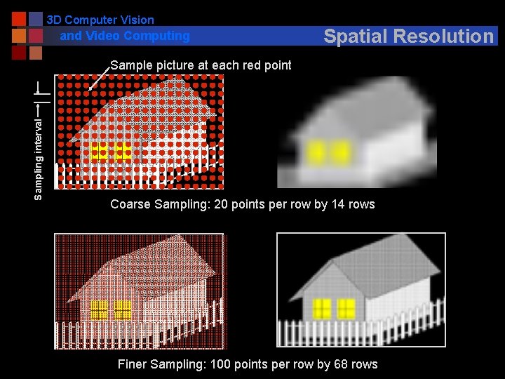
3 D Computer Vision and Video Computing n Digitization: Spatial Resolution Let's digitize this image l l Assume a square sampling pattern Vary density of sampling grid

3 D Computer Vision and Video Computing n Effect of Sampling Interval - 1 Look in vicinity of the picket fence: Sampling Interval: NO EVIDENCE OF THE FENCE! White Image! Dark Gray Image!

3 D Computer Vision and Video Computing n Effect of Sampling Interval - 2 Look in vicinity of picket fence: Sampling Interval: What's the difference between this attempt and the last one? Now we've got a fence!

3 D Computer Vision and Video Computing n The Missing Fence Found Consider the repetitive structure of the fence: Sampling Intervals Case 1: s' = d Case 2: s = d/2 The sampling interval is equal to the size of the repetitive structure The sampling interval is one-half the size of the repetitive structure NO FENCE

3 D Computer Vision and Video Computing n n IF: the size of the smallest structure to be preserved is d THEN: the sampling interval must be smaller than d/2 Can be shown to be true mathematically Repetitive structure has a certain frequency ('pickets/foot') l l n The Sampling Theorem To preserve structure must sample at twice the frequency Holds for images, audio CDs, digital television…. Leads naturally to Fourier Analysis (optional)

3 D Computer Vision and Video Computing n Sampling Rough Idea: Ideal Case 23 "Digitized Image" "Continuous Image" Dirac Delta Function 2 D "Comb" d(x, y) = 0 for x = 0, y= 0 d(x, y) dx dy = 1 s f(x, y)d(x-a, y-b) dx dy = f(a, b) d(x-ns, y-ns) for n = 1…. 32 (e. g. )

3 D Computer Vision and Video Computing n Sampling Rough Idea: Actual Case l l l Can't realize an ideal point function in real equipment "Delta function" equivalent has an area Value returned is the average over this area 23 s

3 D Computer Vision and Video Computing Mixed Pixel Problem

3 D Computer Vision and Video Computing n Signal Quantization Goal: determine a mapping from a continuous signal (e. g. analog video signal) to one of K discrete (digital) levels. I(x, y) =. 1583 volts = ? ? Digital value

3 D Computer Vision Quantization and Video Computing n n n I(x, y) = continuous signal: 0 ≤ I ≤ M Want to quantize to K values 0, 1, . . K-1 K usually chosen to be a power of 2: K 2 4 8 16 32 64 128 256 n n #Levels 2 4 8 16 32 64 128 256 #Bits 1 2 3 4 5 6 7 8 Mapping from input signal to output signal is to be determined. Several types of mappings: uniform, logarithmic, etc.

3 D Computer Vision Choice of K and Video Computing Original K=2 K=4 K=16 K=32 Linear Ramp

3 D Computer Vision and Video Computing Choice of K K=2 (each color) K=4 (each color)

3 D Computer Vision and Video Computing n n Choice of Function: Uniform sampling divides the signal range [0 -M] into K equal-sized intervals. The integers 0, . . . K-1 are assigned to these intervals. All signal values within an interval are represented by the associated integer value. Defines a mapping:

3 D Computer Vision and Video Computing n n n Logarithmic Quantization Signal is log I(x, y). Effect is: Detail enhanced in the low signal values at expense of detail in high signal values.

3 D Computer Vision and Video Computing Logarithmic Quantization Curve Original Logarithmic Quantization

3 D Computer Vision and Video Computing Hexagonal Rectangular Tesselation Patterns Triangular Typical

3 D Computer Vision Digital Geometry and Video Computing I(i, j) (0, 0) j Picture Element or Pixel i 32 n n n Neighborhood Connectedness Distance Metrics Pixel value I(I, j) = 0, 1 Binary Image 0 - K-1 Gray Scale Image Vector: Multispectral Image

3 D Computer Vision and Video Computing n n Connected Components Binary image with multiple 'objects' Separate 'objects' must be labeled individually 6 Connected Components

3 D Computer Vision and Video Computing Finding n Connected Components Two points in an image are 'connected' if a path can be found for which the value of the image function is the same all along the path. P 1 connected to P 2 P 3 connected to P 4 P 1 not connected to P 3 or P 4 P 2 not connected to P 3 or P 4 P 3 not connected to P 1 or P 2 P 4 not connected to P 1 or P 2

3 D Computer Vision and Video Computing n n n Algorithm Pick any pixel in the image and assign it a label Assign same label to any neighbor pixel with the same value of the image function Continue labeling neighbors until no neighbors can be assigned this label Choose another label and another pixel not already labeled and continue If no more unlabeled image points, stop. Who's my neighbor?

3 D Computer Vision and Video Computing Example

3 D Computer Vision Neighbor and Video Computing n n Consider the definition of the term 'neighbor' Two common definitions: Four Neighbor n n Eight Neighbor Consider what happens with a closed curve. One would expect a closed curve to partition the plane into two connected regions.

3 D Computer Vision and Video Computing Alternate Neighborhood Definitions

3 D Computer Vision and Video Computing n Use 4 -neighborhood for object and 8 -neighborhood for background l n Possible Solutions requires a-priori knowledge about which pixels are object and which are background Use a six-connected neighborhood:

3 D Computer Vision Digital Distances and Video Computing n Alternate distance metrics for digital images Euclidean Distance = (i-n) 2 + (j-m) 2 City Block Distance = |i-n| + |j-m| Chessboard Distance = max[ |i-n|, |j-m| ]

3 D Computer Vision and Video Computing Next: Camera Models n Homework #1 online, Due Feb 22 Tue before midnight Next