3 D Computer Vision 3 D Vision and

3 D Computer Vision 3 D Vision and Video Computing CSc I 6716 Fall 2005 Topic 3 of Part II Calibration Zhigang Zhu, City College of New York zhu@cs. ccny. cuny. edu

3 D Computer Vision and Video Computing n Calibration: Find the intrinsic and extrinsic parameters l l l n l Basic equations (from Lecture 5) Estimating the Image center using vanishing points l SVD (Singular Value Decomposition) and Homogeneous System l Focal length, Aspect ratio, and extrinsic parameters l Discussion: Why not do all the parameters together? Projection Matrix Approach (…after-class reading) l l l n Problem and assumptions Direct parameter estimation approach Projection matrix approach Direct Parameter Estimation Approach l n Lecture Outline Estimating the projection matrix M Computing the camera parameters from M Discussion Comparison and Summary l Any difference?

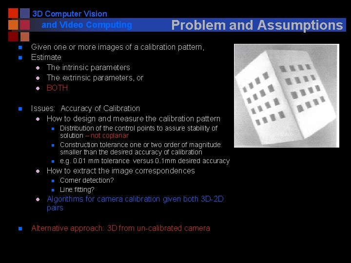
3 D Computer Vision and Video Computing n n n Given one or more images of a calibration pattern, Estimate l The intrinsic parameters l The extrinsic parameters, or l BOTH Issues: Accuracy of Calibration l How to design and measure the calibration pattern n l n l Distribution of the control points to assure stability of solution – not coplanar Construction tolerance one or two order of magnitude smaller than the desired accuracy of calibration e. g. 0. 01 mm tolerance versus 0. 1 mm desired accuracy How to extract the image correspondences n n Problem and Assumptions Corner detection? Line fitting? Algorithms for camera calibration given both 3 D-2 D pairs Alternative approach: 3 D from un-calibrated camera

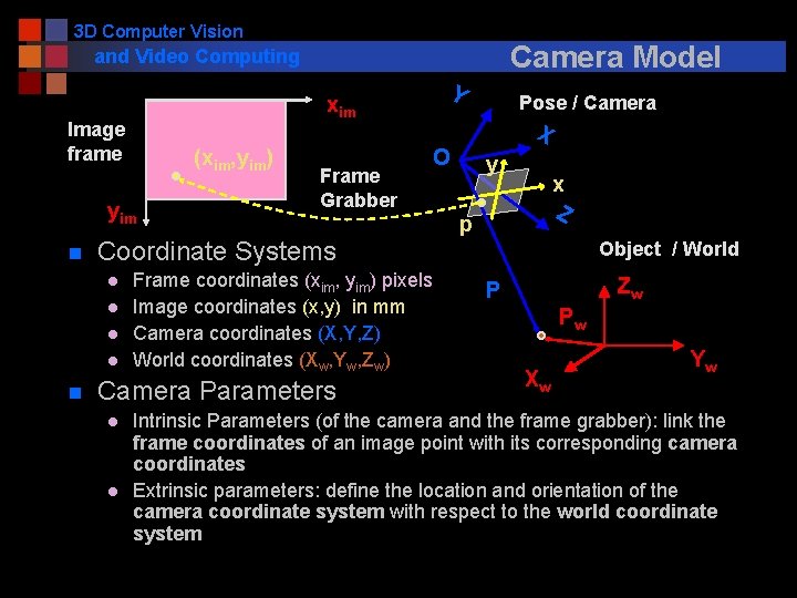
3 D Computer Vision Camera Model and Video Computing xim Image frame (xim, yim) yim n Coordinate Systems l l n Frame Grabber Frame coordinates (xim, yim) pixels Image coordinates (x, y) in mm Camera coordinates (X, Y, Z) World coordinates (Xw, Yw, Zw) Camera Parameters l l Y Pose / Camera X O y x Z p Object / World Zw P Pw Xw Yw Intrinsic Parameters (of the camera and the frame grabber): link the frame coordinates of an image point with its corresponding camera coordinates Extrinsic parameters: define the location and orientation of the camera coordinate system with respect to the world coordinate system

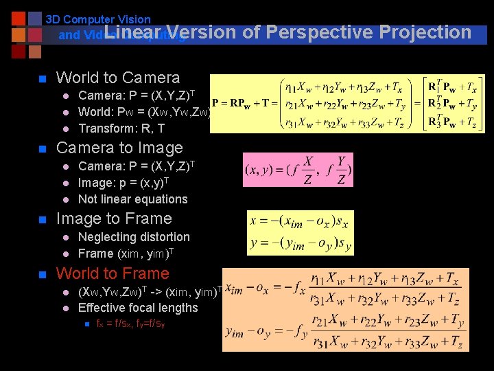
3 D Computer Vision Linear Version and Video Computing n World to Camera l l l n Camera to Image l l l n Camera: P = (X, Y, Z)T Image: p = (x, y)T Not linear equations Image to Frame l l n Camera: P = (X, Y, Z)T World: Pw = (Xw, Yw, Zw)T Transform: R, T Neglecting distortion Frame (xim, yim)T World to Frame l l (Xw, Yw, Zw)T -> (xim, yim)T Effective focal lengths n fx = f/sx, fy=f/sy of Perspective Projection

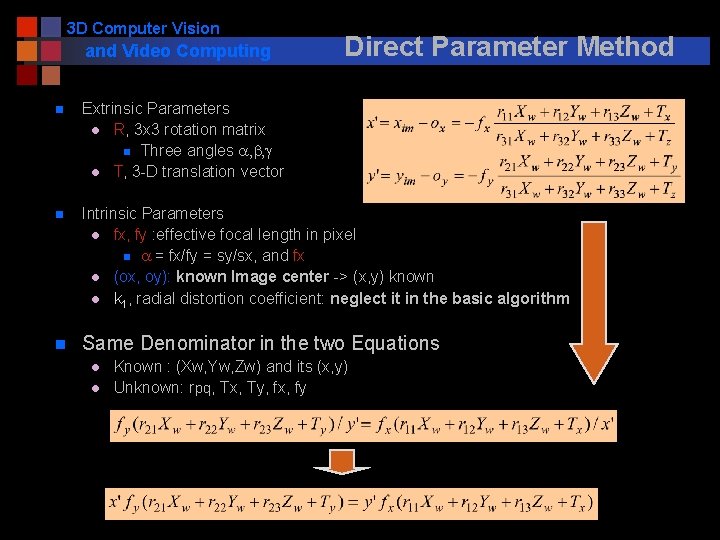
3 D Computer Vision and Video Computing Direct Parameter Method n Extrinsic Parameters l R, 3 x 3 rotation matrix n Three angles a, b, g l T, 3 -D translation vector n Intrinsic Parameters l fx, fy : effective focal length in pixel n a = fx/fy = sy/sx, and fx l (ox, oy): known Image center -> (x, y) known l k 1, radial distortion coefficient: neglect it in the basic algorithm n Same Denominator in the two Equations l l Known : (Xw, Yw, Zw) and its (x, y) Unknown: rpq, Tx, Ty, fx, fy

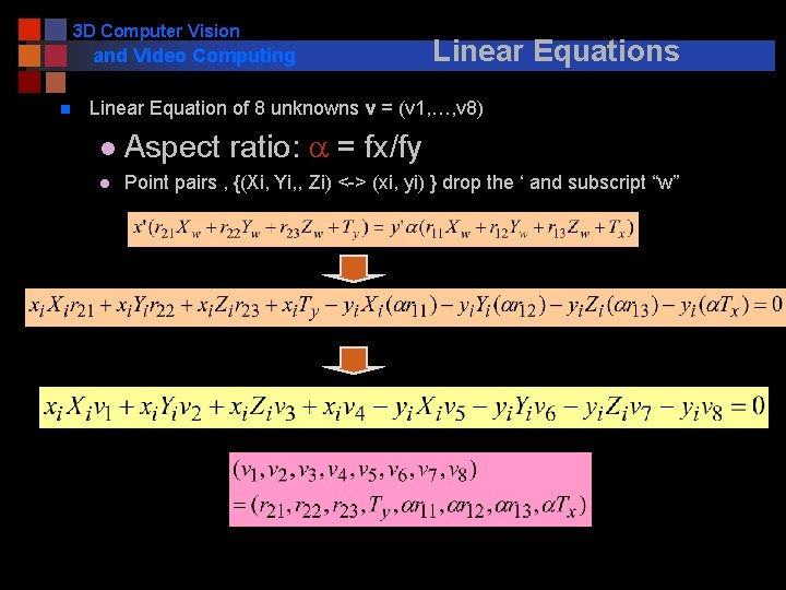
3 D Computer Vision and Video Computing n Linear Equations Linear Equation of 8 unknowns v = (v 1, …, v 8) l Aspect ratio: a = fx/fy l Point pairs , {(Xi, Yi, , Zi) <-> (xi, yi) } drop the ‘ and subscript “w”

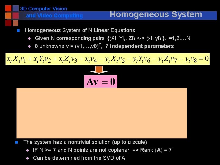
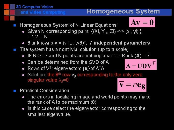
3 D Computer Vision and Video Computing n n Homogeneous System of N Linear Equations l Given N corresponding pairs {(Xi, Yi, , Zi) <-> (xi, yi) }, i=1, 2, …N l 8 unknowns v = (v 1, …, v 8)T, 7 independent parameters The system has a nontrivial solution (up to a scale) l IF N >= 7 and N points are not coplanar => Rank (A) = 7 l Can be determined from the SVD of A

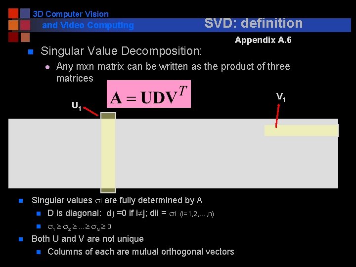
3 D Computer Vision and Video Computing n SVD: definition Singular Value Decomposition: l Any mxn matrix can be written as the product of three matrices U 1 n n Appendix A. 6 Singular values si are fully determined by A n D is diagonal: dij =0 if i j; dii = si (i=1, 2, …, n) n s 1 s 2 … s. N 0 Both U and V are not unique n Columns of each are mutual orthogonal vectors V 1

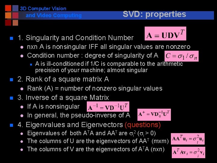
3 D Computer Vision and Video Computing n 1. Singularity and Condition Number l l nxn A is nonsingular IFF all singular values are nonzero Condition number : degree of singularity of A n n Rank (A) = number of nonzero singular values 3. Inverse of a square Matrix l l n A is ill-conditioned if 1/C is comparable to the arithmetic precision of your machine; almost singular 2. Rank of a square matrix A l n SVD: properties If A is nonsingular In general, the pseudo-inverse of A 4. Eigenvalues and Eigenvectors (questions) l l l Eigenvalues of both ATA and AAT are si 2 (si > 0) The columns of U are the eigenvectors of AAT (mxm) The columns of V are the eigenvectors of ATA (nxn)

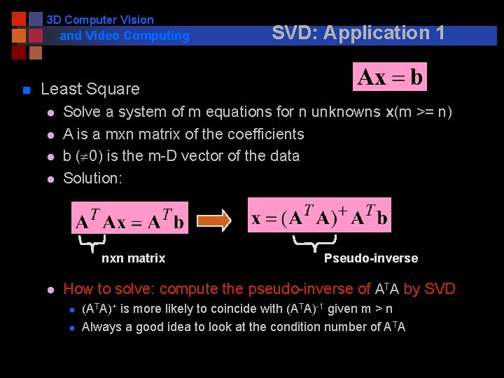
3 D Computer Vision and Video Computing n SVD: Application 1 Least Square l l Solve a system of m equations for n unknowns x(m >= n) A is a mxn matrix of the coefficients b ( 0) is the m-D vector of the data Solution: nxn matrix l Pseudo-inverse How to solve: compute the pseudo-inverse of ATA by SVD n n (ATA)+ is more likely to coincide with (ATA)-1 given m > n Always a good idea to look at the condition number of ATA

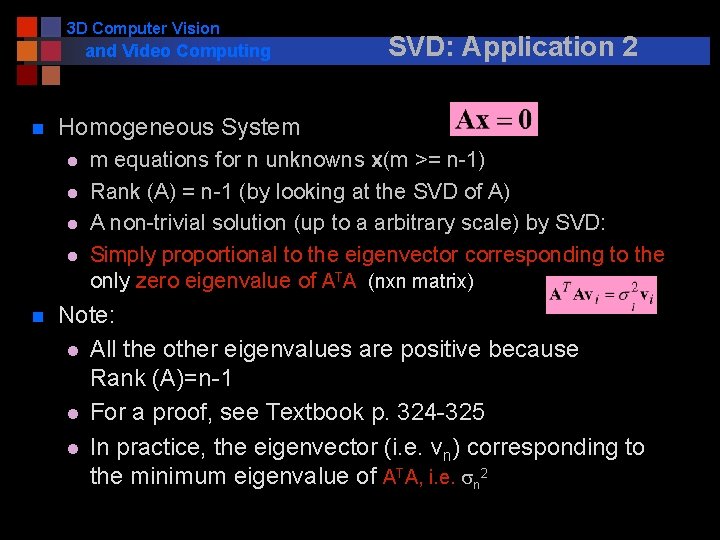
3 D Computer Vision and Video Computing n Homogeneous System l l n SVD: Application 2 m equations for n unknowns x(m >= n-1) Rank (A) = n-1 (by looking at the SVD of A) A non-trivial solution (up to a arbitrary scale) by SVD: Simply proportional to the eigenvector corresponding to the only zero eigenvalue of ATA (nxn matrix) Note: l All the other eigenvalues are positive because Rank (A)=n-1 l For a proof, see Textbook p. 324 -325 l In practice, the eigenvector (i. e. vn) corresponding to the minimum eigenvalue of ATA, i. e. sn 2

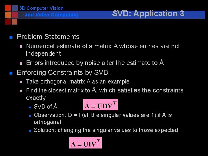
3 D Computer Vision and Video Computing n Problem Statements l l n SVD: Application 3 Numerical estimate of a matrix A whose entries are not independent Errors introduced by noise alter the estimate to Enforcing Constraints by SVD l Take orthogonal matrix A as an example l Find the closest matrix to , which satisfies the constraints exactly n n n SVD of Observation: D = I (all the singular values are 1) if A is orthogonal Solution: changing the singular values to those expected

3 D Computer Vision and Video Computing n n n Homogeneous System of N Linear Equations l Given N corresponding pairs {(Xi, Yi, , Zi) <-> (xi, yi) }, i=1, 2, …N l 8 unknowns v = (v 1, …, v 8)T, 7 independent parameters The system has a nontrivial solution (up to a scale) l IF N >= 7 and N points are not coplanar => Rank (A) = 7 l Can be determined from the SVD of A l Rows of VT: eigenvectors {ei} of ATA l Solution: the 8 th row e 8 corresponding to the only zero singular value l 8=0 Practical Consideration l The errors in localizing image and world points may make the rank of A to be maximum (8) l In this case select the eigenvector corresponding to the smallest eigenvalue.

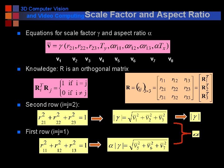
3 D Computer Vision and Video Computing Scale n Factor and Aspect Ratio Equations for scale factor g and aspect ratio a v 1 v 2 v 3 v 4 v 5 n Knowledge: R is an orthogonal matrix n Second row (i=j=2): n First row (i=j=1) v 6 v 7 v 8

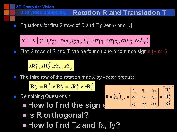
3 D Computer Vision and Video Computing Rotation R and Translation T n Equations for first 2 rows of R and T given a and |g| n First 2 rows of R and T can be found up to a common sign s (+ or -) n The third row of the rotation matrix by vector product n Remaining Questions : l How to find the sign s? l Is R orthogonal? l How to find Tz and fx, fy?

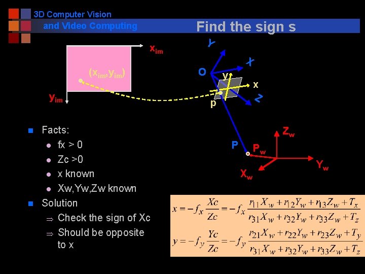
3 D Computer Vision Find the sign s and Video Computing xim (xim, yim) yim n n Facts: l fx > 0 l Zc >0 l x known l Xw, Yw, Zw known Solution Þ Check the sign of Xc Þ Should be opposite to x Y X O y x Z p Zw P Pw Xw Yw

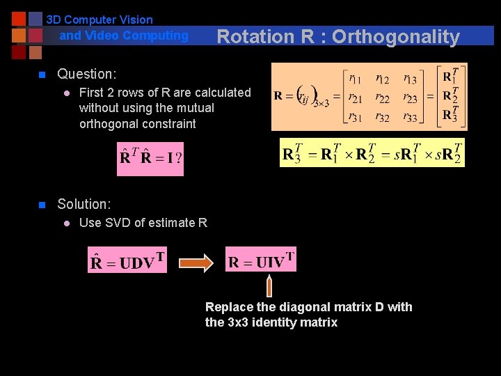
3 D Computer Vision Rotation R : Orthogonality and Video Computing n Question: l n First 2 rows of R are calculated without using the mutual orthogonal constraint Solution: l Use SVD of estimate R Replace the diagonal matrix D with the 3 x 3 identity matrix

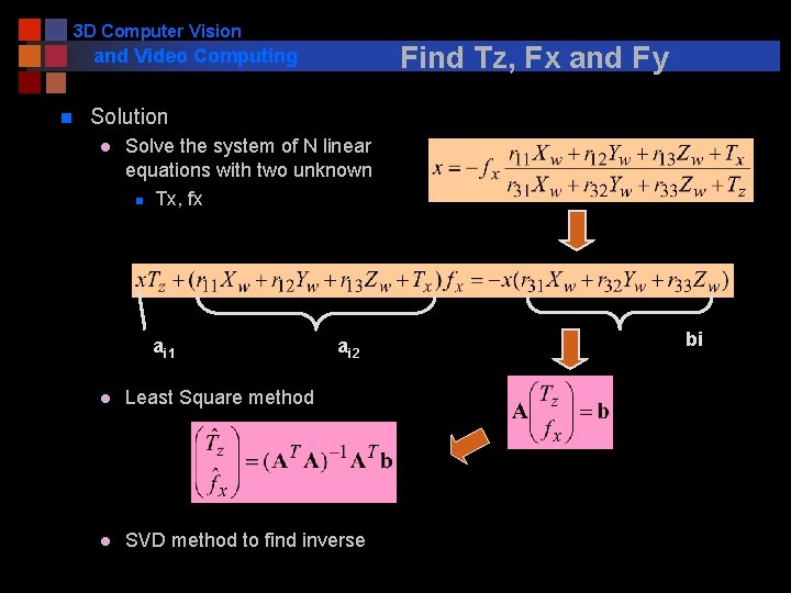
3 D Computer Vision Find Tz, Fx and Fy and Video Computing n Solution l Solve the system of N linear equations with two unknown n Tx, fx ai 1 ai 2 l Least Square method l SVD method to find inverse bi

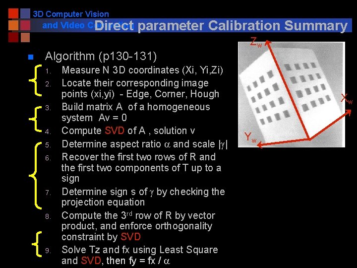
3 D Computer Vision and Video Computing Direct n parameter Calibration Summary Algorithm (p 130 -131) 1. 2. 3. 4. 5. 6. 7. 8. 9. Measure N 3 D coordinates (Xi, Yi, Zi) Locate their corresponding image points (xi, yi) - Edge, Corner, Hough Build matrix A of a homogeneous system Av = 0 Compute SVD of A , solution v Determine aspect ratio a and scale |g| Recover the first two rows of R and the first two components of T up to a sign Determine sign s of g by checking the projection equation Compute the 3 rd row of R by vector product, and enforce orthogonality constraint by SVD Solve Tz and fx using Least Square and SVD, then fy = fx / a Zw Xw Yw

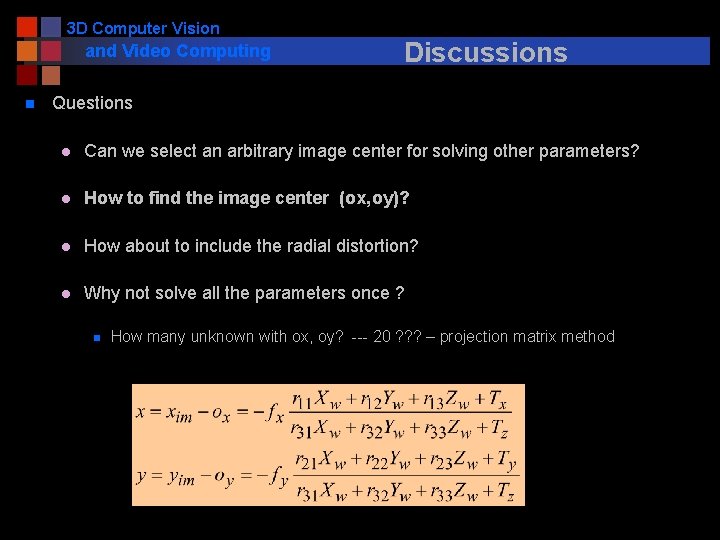
3 D Computer Vision and Video Computing n Discussions Questions l Can we select an arbitrary image center for solving other parameters? l How to find the image center (ox, oy)? l How about to include the radial distortion? l Why not solve all the parameters once ? n How many unknown with ox, oy? --- 20 ? ? ? – projection matrix method

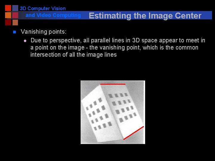
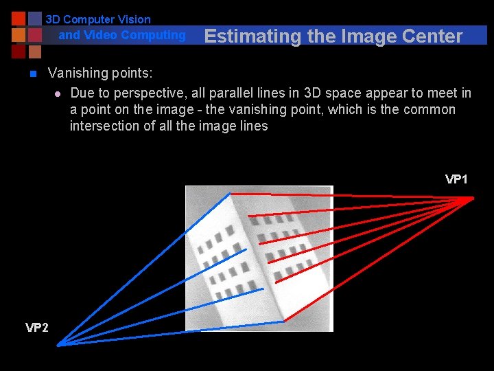
3 D Computer Vision and Video Computing n Estimating the Image Center Vanishing points: l Due to perspective, all parallel lines in 3 D space appear to meet in a point on the image - the vanishing point, which is the common intersection of all the image lines

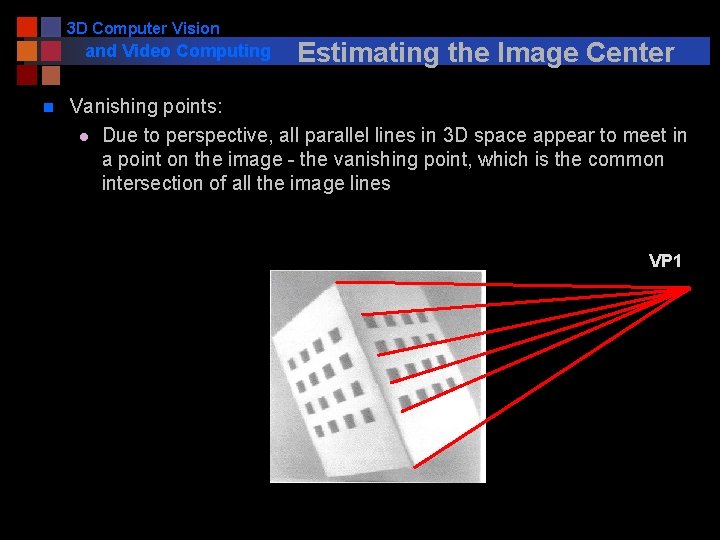
3 D Computer Vision and Video Computing n Estimating the Image Center Vanishing points: l Due to perspective, all parallel lines in 3 D space appear to meet in a point on the image - the vanishing point, which is the common intersection of all the image lines VP 1

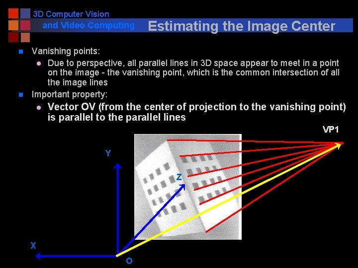
3 D Computer Vision and Video Computing n n Estimating the Image Center Vanishing points: l Due to perspective, all parallel lines in 3 D space appear to meet in a point on the image - the vanishing point, which is the common intersection of all the image lines Important property: l Vector OV (from the center of projection to the vanishing point) is parallel to the parallel lines VP 1 Y Z X O

3 D Computer Vision and Video Computing n Estimating the Image Center Vanishing points: l Due to perspective, all parallel lines in 3 D space appear to meet in a point on the image - the vanishing point, which is the common intersection of all the image lines VP 1 VP 2

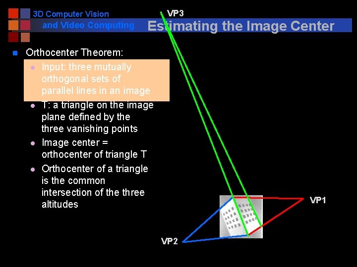
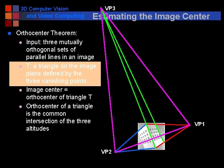
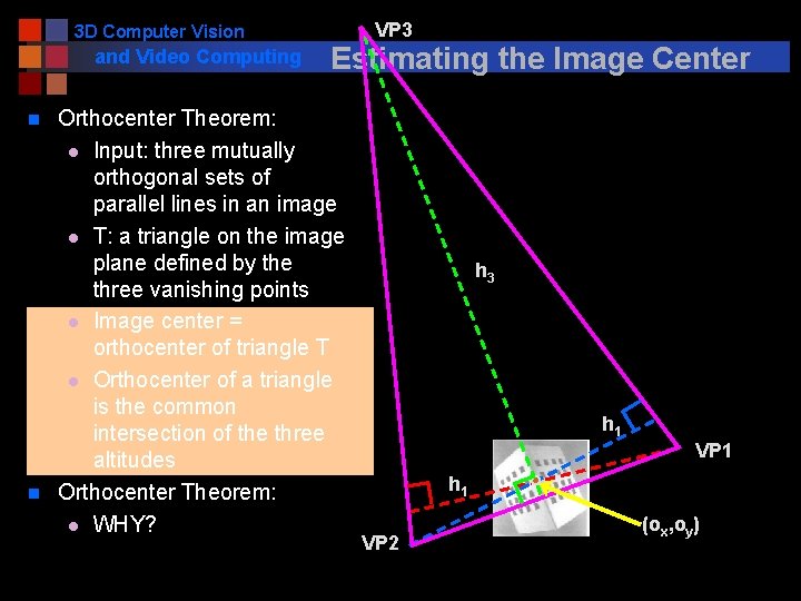
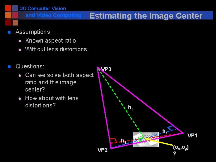
3 D Computer Vision and Video Computing n VP 3 Estimating the Image Center Orthocenter Theorem: l Input: three mutually orthogonal sets of parallel lines in an image l T: a triangle on the image plane defined by the three vanishing points l Image center = orthocenter of triangle T l Orthocenter of a triangle is the common intersection of the three altitudes VP 1 VP 2

3 D Computer Vision and Video Computing n VP 3 Estimating the Image Center Orthocenter Theorem: l Input: three mutually orthogonal sets of parallel lines in an image l T: a triangle on the image plane defined by the three vanishing points l Image center = orthocenter of triangle T l Orthocenter of a triangle is the common intersection of the three altitudes VP 1 VP 2

3 D Computer Vision and Video Computing n n VP 3 Estimating the Image Center Orthocenter Theorem: l Input: three mutually orthogonal sets of parallel lines in an image l T: a triangle on the image plane defined by the three vanishing points l Image center = orthocenter of triangle T l Orthocenter of a triangle is the common intersection of the three altitudes Orthocenter Theorem: l WHY? h 3 h 1 VP 1 h 1 VP 2 (ox, oy)

3 D Computer Vision and Video Computing Estimating the Image Center n Assumptions: l Known aspect ratio l Without lens distortions n Questions: l Can we solve both aspect ratio and the image center? l How about with lens distortions? VP 3 h 1 h 1 VP 2 VP 1 (ox, oy) ?

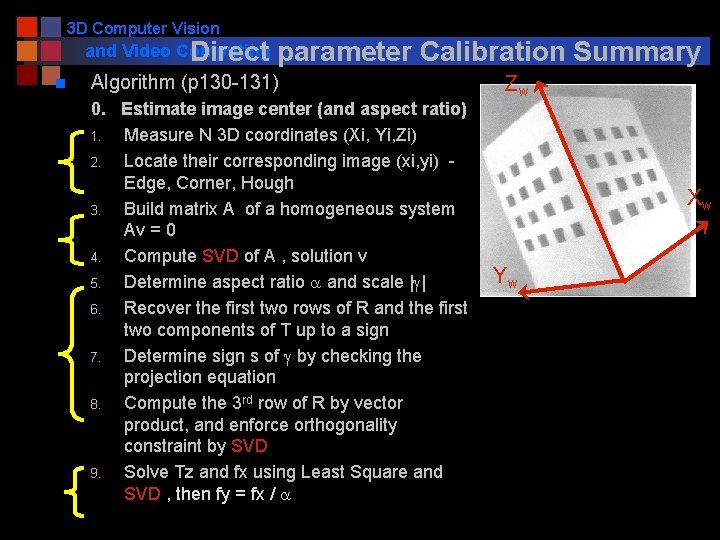
3 D Computer Vision and Video Computing Direct n parameter Calibration Summary Algorithm (p 130 -131) 0. Estimate image center (and aspect ratio) 1. Measure N 3 D coordinates (Xi, Yi, Zi) 2. Locate their corresponding image (xi, yi) Edge, Corner, Hough 3. Build matrix A of a homogeneous system Av = 0 4. Compute SVD of A , solution v 5. Determine aspect ratio a and scale |g| 6. Recover the first two rows of R and the first two components of T up to a sign 7. Determine sign s of g by checking the projection equation 8. Compute the 3 rd row of R by vector product, and enforce orthogonality constraint by SVD 9. Solve Tz and fx using Least Square and SVD , then fy = fx / a Zw Xw Yw

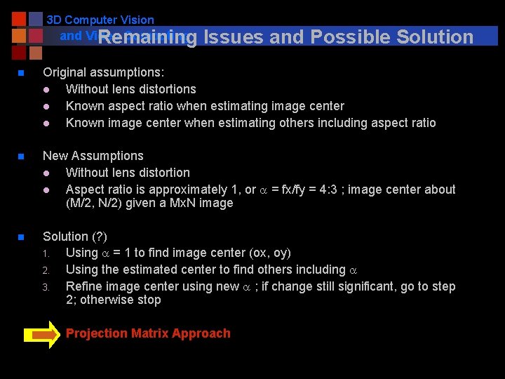
3 D Computer Vision and Video Computing Remaining Issues and Possible Solution n Original assumptions: l Without lens distortions l Known aspect ratio when estimating image center l Known image center when estimating others including aspect ratio n New Assumptions l Without lens distortion l Aspect ratio is approximately 1, or a = fx/fy = 4: 3 ; image center about (M/2, N/2) given a Mx. N image n Solution (? ) 1. Using a = 1 to find image center (ox, oy) 2. Using the estimated center to find others including a 3. Refine image center using new a ; if change still significant, go to step 2; otherwise stop l Projection Matrix Approach

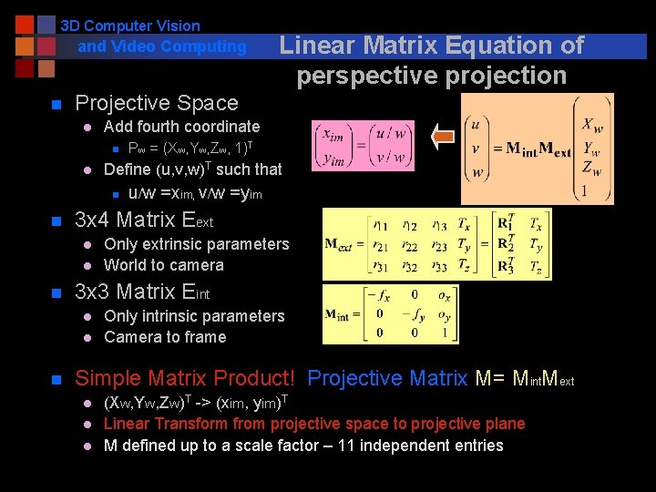
3 D Computer Vision and Video Computing n Projective Space l Add fourth coordinate n l l Only extrinsic parameters World to camera 3 x 3 Matrix Eint l l n u/w =xim, v/w =yim 3 x 4 Matrix Eext l n Pw = (Xw, Yw, Zw, 1)T Define (u, v, w)T such that n n Linear Matrix Equation of perspective projection Only intrinsic parameters Camera to frame Simple Matrix Product! Projective Matrix M= Mint. Mext l l l (Xw, Yw, Zw)T -> (xim, yim)T Linear Transform from projective space to projective plane M defined up to a scale factor – 11 independent entries

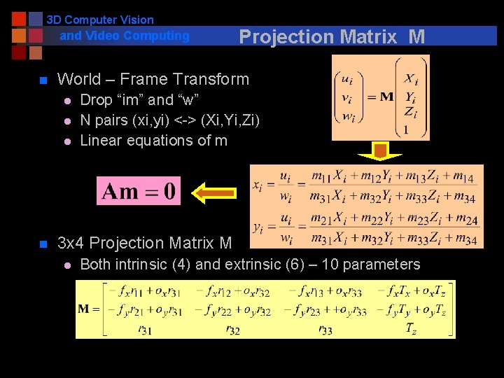
3 D Computer Vision and Video Computing n World – Frame Transform l l l n Projection Matrix M Drop “im” and “w” N pairs (xi, yi) <-> (Xi, Yi, Zi) Linear equations of m 3 x 4 Projection Matrix M l Both intrinsic (4) and extrinsic (6) – 10 parameters

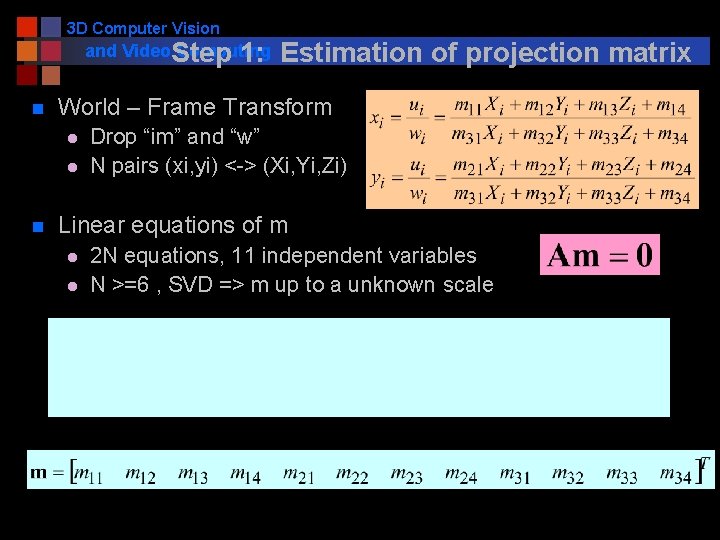
3 D Computer Vision and Video. Step Computing 1: n World – Frame Transform l l n Estimation of projection matrix Drop “im” and “w” N pairs (xi, yi) <-> (Xi, Yi, Zi) Linear equations of m l l 2 N equations, 11 independent variables N >=6 , SVD => m up to a unknown scale

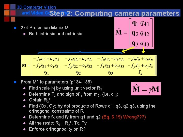
3 D Computer Vision and Video Computing Step 2: Computing camera parameters n 3 x 4 Projection Matrix M l Both intrinsic and extrinsic n From M^ to parameters (p 134 -135) l Find scale |g| by using unit vector R 3 T l Determine Tz and sign of g from m 34 (i. e. q 43) l Obtain R 3 T l Find (Ox, Oy) by dot products of Rows q 1. q 3, q 2. q 3, using the orthogonal constraints of R l Determine fx and fy from q 1 and q 2 (Eq. 6. 19) Wrong? ? ? ) l All the rests: R 1 T, R 2 T, Tx, Ty l Enforce orthognoality on R?

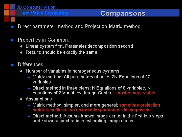
3 D Computer Vision and Video Computing Comparisons n Direct parameter method and Projection Matrix method n Properties in Common: l l n Linear system first, Parameter decomposition second Results should be exactly the same Differences l l Number of variables in homogeneous systems n Matrix method: All parameters at once, 2 N Equations of 12 variables n Direct method in three steps: N Equations of 8 variables, N equations of 2 Variables, Image Center – maybe more stable Assumptions n Matrix method: simpler, and more general; sometime projection matrix is sufficient so no need for parameter decompostion n Direct method: Assume known image center in the first two steps, and known aspect ratio in estimating image center

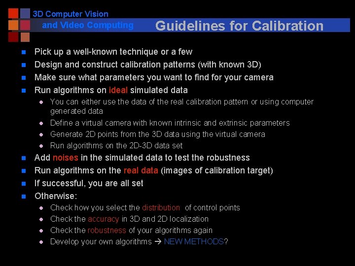
3 D Computer Vision and Video Computing n n Pick up a well-known technique or a few Design and construct calibration patterns (with known 3 D) Make sure what parameters you want to find for your camera Run algorithms on ideal simulated data l l n n Guidelines for Calibration You can either use the data of the real calibration pattern or using computer generated data Define a virtual camera with known intrinsic and extrinsic parameters Generate 2 D points from the 3 D data using the virtual camera Run algorithms on the 2 D-3 D data set Add noises in the simulated data to test the robustness Run algorithms on the real data (images of calibration target) If successful, you are all set Otherwise: l l Check how you select the distribution of control points Check the accuracy in 3 D and 2 D localization Check the robustness of your algorithms again Develop your own algorithms NEW METHODS?

3 D Computer Vision and Video Computing n 3 D reconstruction using two cameras Stereo Vision Next