3 Chapter 4 Describing the Relation between Two

Section 4. 4 Contingency Tables and Association © 2010 Pearson Prentice Hall. All rights

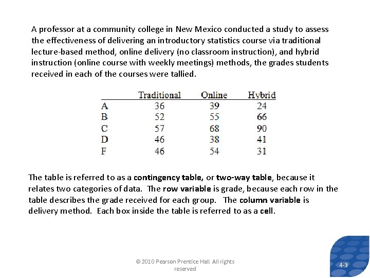
A professor at a community college in New Mexico conducted a study to assess the effectiveness of delivering an introductory statistics course via traditional lecture-based method, online delivery (no classroom instruction), and hybrid instruction (online course with weekly meetings) methods, the grades students received in each of the courses were tallied. The table is referred to as a contingency table, or two-way table, because it relates two categories of data. The row variable is grade, because each row in the table describes the grade received for each group. The column variable is delivery method. Each box inside the table is referred to as a cell. © 2010 Pearson Prentice Hall. All rights reserved 3 4 -3

© 2010 Pearson Prentice Hall. All rights reserved 4 -4 4

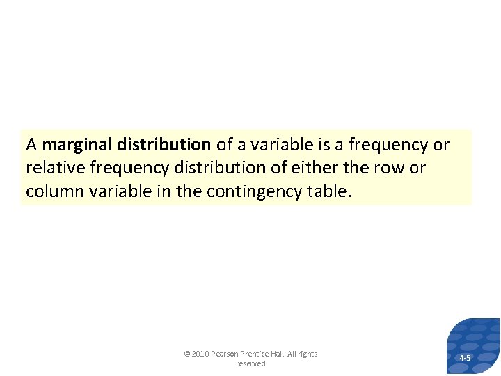
A marginal distribution of a variable is a frequency or relative frequency distribution of either the row or column variable in the contingency table. © 2010 Pearson Prentice Hall. All rights reserved 4 -5 5

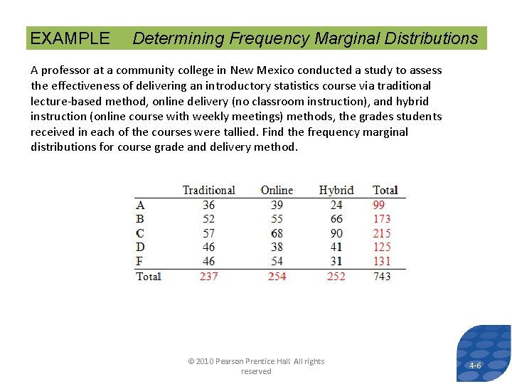
EXAMPLE Determining Frequency Marginal Distributions A professor at a community college in New Mexico conducted a study to assess the effectiveness of delivering an introductory statistics course via traditional lecture-based method, online delivery (no classroom instruction), and hybrid instruction (online course with weekly meetings) methods, the grades students received in each of the courses were tallied. Find the frequency marginal distributions for course grade and delivery method. © 2010 Pearson Prentice Hall. All rights reserved 4 -6 6

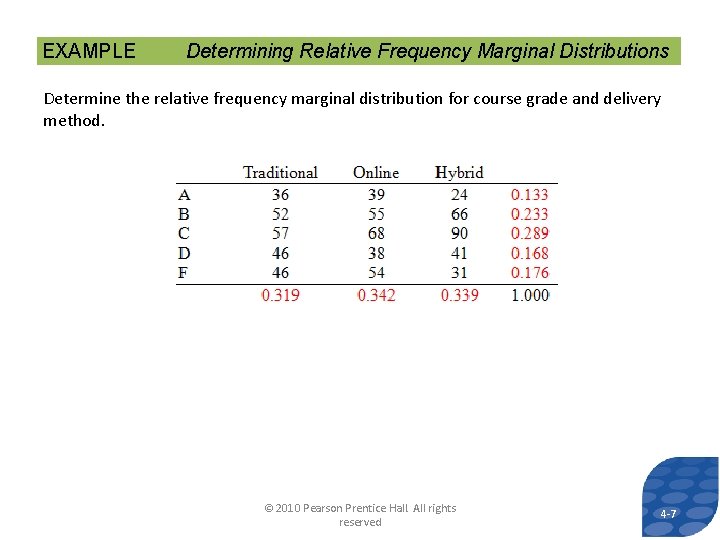
EXAMPLE Determining Relative Frequency Marginal Distributions Determine the relative frequency marginal distribution for course grade and delivery method. © 2010 Pearson Prentice Hall. All rights reserved 4 -7 7

© 2010 Pearson Prentice Hall. All rights reserved 4 -8 8

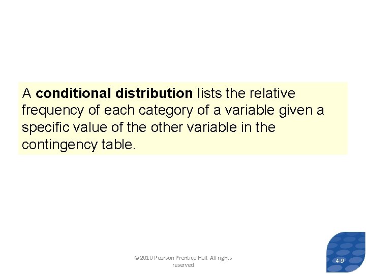
A conditional distribution lists the relative frequency of each category of a variable given a specific value of the other variable in the contingency table. © 2010 Pearson Prentice Hall. All rights reserved 4 -9 9

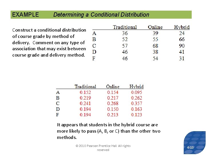
EXAMPLE Determining a Conditional Distribution Construct a conditional distribution of course grade by method of delivery. Comment on any type of association that may exist between course grade and delivery method. It appears that students in the hybrid course are more likely to pass (A, B, or C) than the other two methods. © 2010 Pearson Prentice Hall. All rights reserved 4 -10 10

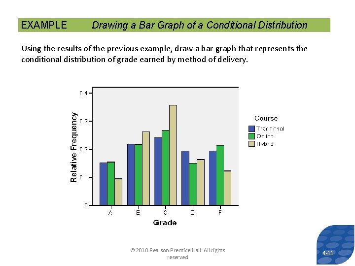
EXAMPLE Drawing a Bar Graph of a Conditional Distribution Using the results of the previous example, draw a bar graph that represents the conditional distribution of grade earned by method of delivery. © 2010 Pearson Prentice Hall. All rights reserved 4 -11 11

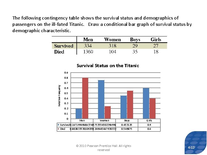
The following contingency table shows the survival status and demographics of passengers on the ill-fated Titanic. Draw a conditional bar graph of survival status by demographic characteristic. Survival Status on the Titanic 0. 9 0. 8 Relative Frequeny 0. 7 0. 6 0. 5 0. 4 0. 3 0. 2 0. 1 0 Men Women Survived 0. 197166469893743 0. 753554502369669 Died 0. 802833530106257 0. 246445497630332 Boys 0. 453125 0. 546875 © 2010 Pearson Prentice Hall. All rights reserved Girls 0. 6 0. 4 4 -12 12

© 2010 Pearson Prentice Hall. All rights reserved 4 -13 13

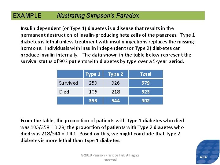
EXAMPLE Illustrating Simpson’s Paradox Insulin dependent (or Type 1) diabetes is a disease that results in the permanent destruction of insulin-producing beta cells of the pancreas. Type 1 diabetes is lethal unless treatment with insulin injections replaces the missing hormone. Individuals with insulin independent (or Type 2) diabetes can produce insulin internally. The data shown in the table below represent the survival status of 902 patients with diabetes by type over a 5 -year period. Type 1 Type 2 Total Survived 253 326 579 Died 105 218 323 358 544 902 From the table, the proportion of patients with Type 1 diabetes who died was 105/358 = 0. 29; the proportion of patients with Type 2 diabetes who died was 218/544 = 0. 40. Based on this, we might conclude that Type 2 diabetes is more lethal than Type 1 diabetes. © 2010 Pearson Prentice Hall. All rights reserved 4 -14 14

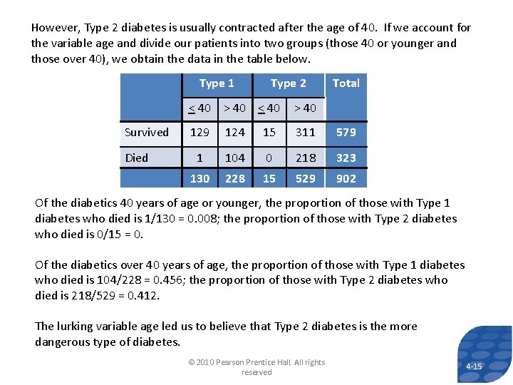
However, Type 2 diabetes is usually contracted after the age of 40. If we account for the variable age and divide our patients into two groups (those 40 or younger and those over 40), we obtain the data in the table below. Type 1 Survived Died Type 2 Total < 40 > 40 129 124 15 311 579 1 104 0 218 323 130 228 15 529 902 Of the diabetics 40 years of age or younger, the proportion of those with Type 1 diabetes who died is 1/130 = 0. 008; the proportion of those with Type 2 diabetes who died is 0/15 = 0. Of the diabetics over 40 years of age, the proportion of those with Type 1 diabetes who died is 104/228 = 0. 456; the proportion of those with Type 2 diabetes who died is 218/529 = 0. 412. The lurking variable age led us to believe that Type 2 diabetes is the more dangerous type of diabetes. © 2010 Pearson Prentice Hall. All rights reserved 4 -15 15

Simpson’s Paradox represents a situation in which an association between two variables inverts or goes away when a third variable is introduced to the analysis. © 2010 Pearson Prentice Hall. All rights reserved 4 -16 16