3 4 Linear Programming What is a Linear

3. 4 Linear Programming

What is a Linear Program? § A linear program is a mathematical model that indicates the goal and requirements of an allocation problem. § It has two or more non-negative variables. § Its objective is expressed as a mathematical function. The objective function plots as a line on a two-dimensional graph. § There are constraints that affect possible levels of the variables. In two dimensions these plot as lines and ordinarily define areas in which the solution must lie. 2

Properties of LP Models 1) Seek to minimize or maximize 2) Include “constraints” or limitations 3) There must be alternatives available 4) All equations are linear

Example LP Model Formulation: The Product Mix Problem Decision: How much to make of > 2 products? Objective: Maximize profit Constraints: Limited resources

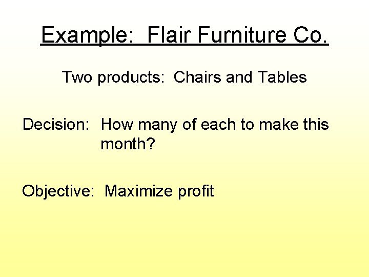
Example: Flair Furniture Co. Two products: Chairs and Tables Decision: How many of each to make this month? Objective: Maximize profit

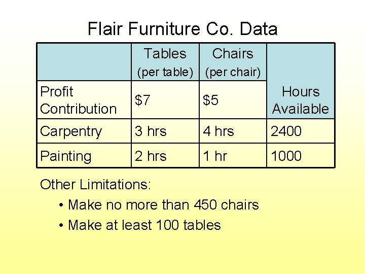
Flair Furniture Co. Data Tables Chairs (per table) (per chair) Profit Contribution $7 $5 Hours Available Carpentry 3 hrs 4 hrs 2400 Painting 2 hrs 1 hr 1000 Other Limitations: • Make no more than 450 chairs • Make at least 100 tables

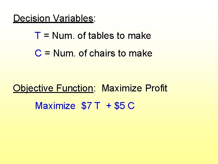
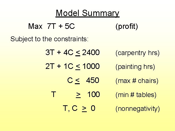
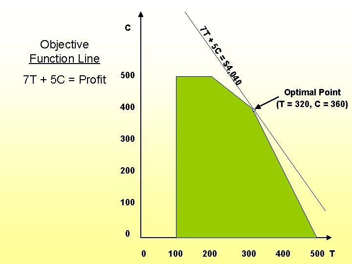
Decision Variables: T = Num. of tables to make C = Num. of chairs to make Objective Function: Maximize Profit Maximize $7 T + $5 C

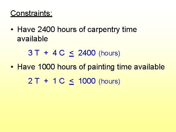
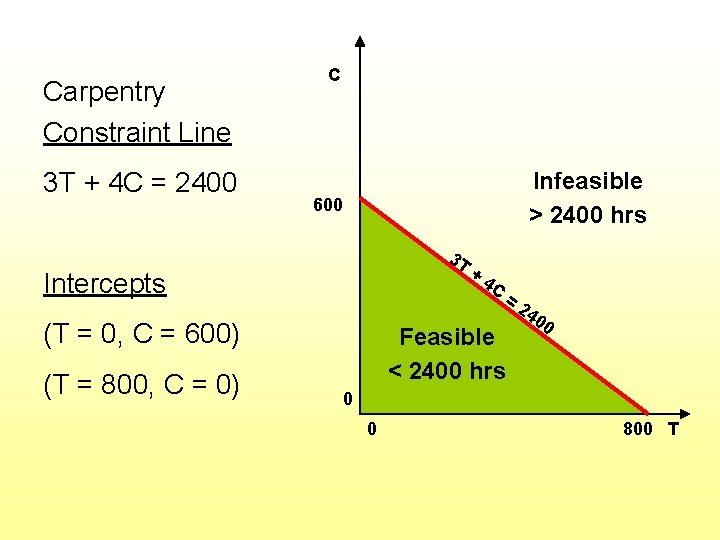
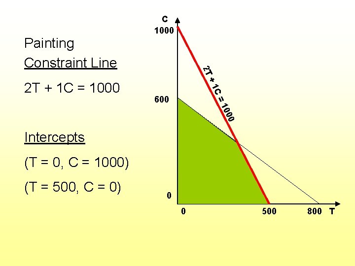
Constraints: • Have 2400 hours of carpentry time available 3 T + 4 C < 2400 (hours) • Have 1000 hours of painting time available 2 T + 1 C < 1000 (hours)

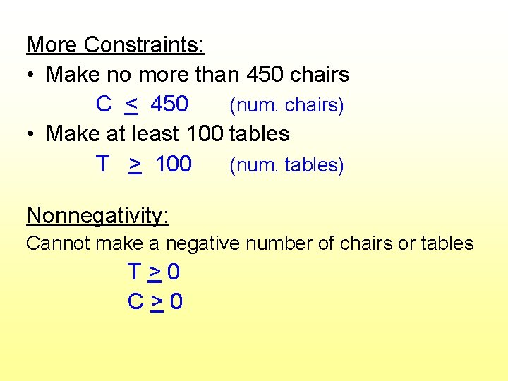
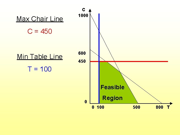
More Constraints: • Make no more than 450 chairs C < 450 (num. chairs) • Make at least 100 tables T > 100 (num. tables) Nonnegativity: Cannot make a negative number of chairs or tables T>0 C>0

Model Summary Max 7 T + 5 C (profit) Subject to the constraints: 3 T + 4 C < 2400 (carpentry hrs) 2 T + 1 C < 1000 (painting hrs) T C < 450 (max # chairs) > 100 (min # tables) T, C > 0 (nonnegativity)

Graphical Solution • Graphing an LP model helps provide insight into LP models and their solutions. • While this can only be done in two dimensions, the same properties apply to all LP models and solutions.

Carpentry Constraint Line 3 T + 4 C = 2400 C Infeasible > 2400 hrs 600 3 T Intercepts (T = 0, C = 600) (T = 800, C = 0) + 4 C = Feasible < 2400 hrs 24 00 0 0 800 T

1 C 2 T + 1 C = 1000 + 2 T Painting Constraint Line C 1000 =1 600 Intercepts (T = 0, C = 1000) (T = 500, C = 0) 0 0 500 800 T

Max Chair Line C 1000 C = 450 Min Table Line 600 450 T = 100 Feasible 0 Region 0 100 500 800 T

+ 7 T C 4 4, 0 =$ 500 0 7 T + 5 C = Profit 5 C Objective Function Line Optimal Point (T = 320, C = 360) 400 300 200 100 0 0 100 200 300 400 500 T

Finding Most Attractive Corner § The optimal solution will always correspond to a corner point of the feasible solution region. § Because there can be many corners, the most attractive corner is easiest to find visually. § That is done by plotting two P lines for arbitrary profit levels. 16

LP Characteristics • Feasible Region: The set of points that satisfies all constraints • Corner Point Property: An optimal solution must lie at one or more corner points • Optimal Solution: The corner point with the best objective function value is optimal

• Because graphs can be inaccurate due to human error and often the numbers are very large or very small it is best to identify the corner point through a system of equations. Simply identify which lines intersect to form the corner point and solve them simultaneously.

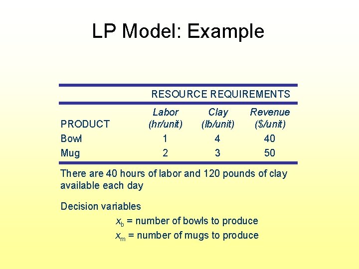
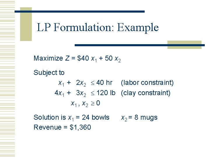
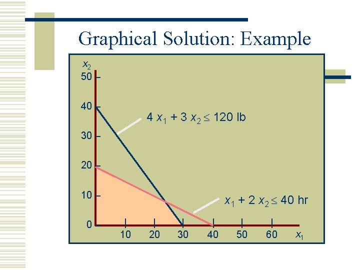
LP Model: Example RESOURCE REQUIREMENTS PRODUCT Bowl Mug Labor (hr/unit) 1 2 Clay (lb/unit) 4 3 Revenue ($/unit) 40 50 There are 40 hours of labor and 120 pounds of clay available each day Decision variables xb = number of bowls to produce xm = number of mugs to produce

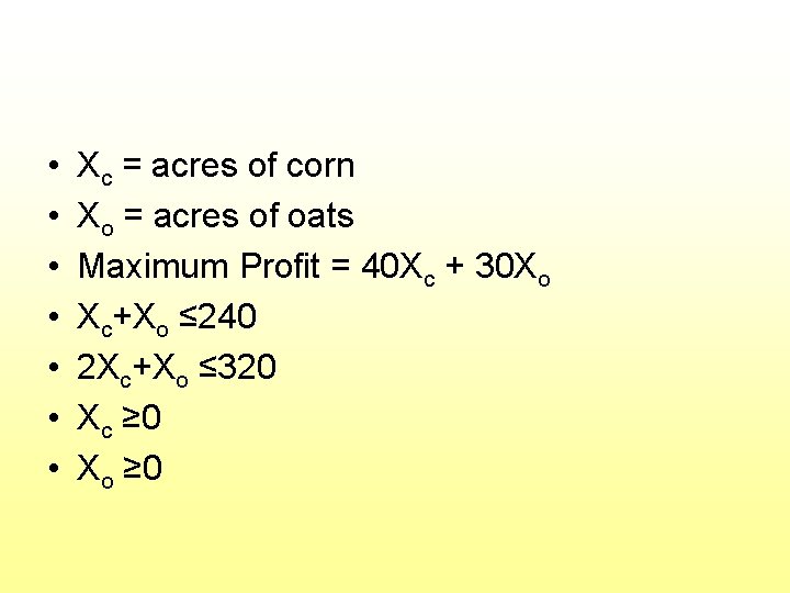
• We have 240 acres of land to plant corn and oats. We make a profit of $40 per acre of corn and $30 per acre of oats. We have 320 hours of available labor. Corn takes 2 hours to plant per acre and oats require 1 hour. How many acres of each should we plant to maximize our profits?

• • Xc = acres of corn Xo = acres of oats Maximum Profit = 40 Xc + 30 Xo Xc+Xo ≤ 240 2 Xc+Xo ≤ 320 Xc ≥ 0 Xo ≥ 0

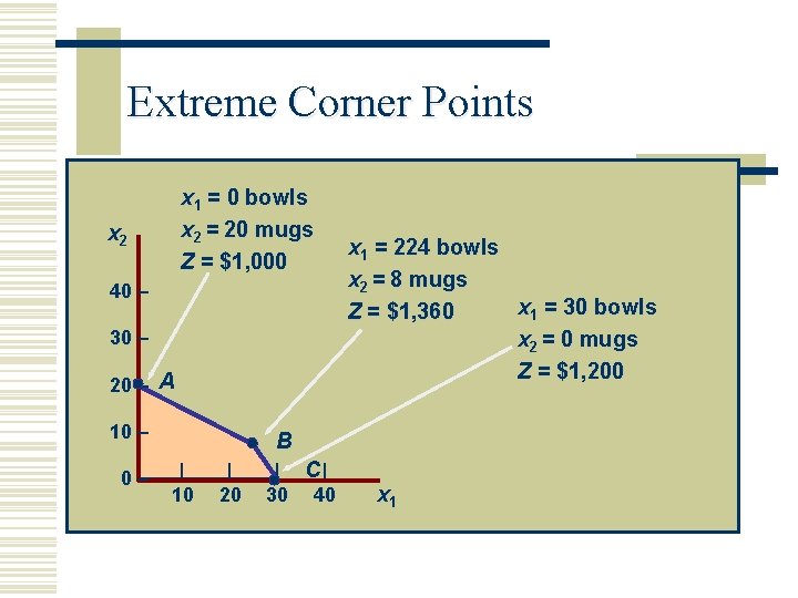
LP Formulation: Example Maximize Z = $40 x 1 + 50 x 2 Subject to x 1 + 2 x 2 4 x 1 + 3 x 2 x 1 , x 2 40 hr (labor constraint) 120 lb (clay constraint) 0 Solution is x 1 = 24 bowls Revenue = $1, 360 x 2 = 8 mugs

Graphical Solution: Example x 2 50 – 4 x 1 + 3 x 2 120 lb 30 – 20 – 10 – 0– x 1 + 2 x 2 40 hr | 10 | 20 | 30 | 40 | 50 | 60 x 1

Extreme Corner Points x 1 = 0 bowls x 2 = 20 mugs Z = $1, 000 x 2 40 – 30 – 20 – A 10 – 0– x 1 = 224 bowls x 2 = 8 mugs x 1 = 30 bowls Z = $1, 360 x 2 = 0 mugs Z = $1, 200 B | 10 | 20 | C| 30 40 x 1

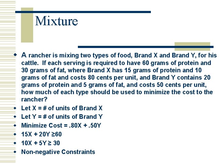
Mixture w A rancher is mixing two types of food, Brand X and Brand Y, for his w w w cattle. If each serving is required to have 60 grams of protein and 30 grams of fat, where Brand X has 15 grams of protein and 10 grams of fat and costs 80 cents per unit, and Brand Y contains 20 grams of protein and 5 grams of fat, and costs 50 cents per unit, how much of each type should be used to minimize the cost to the rancher? Let X = # of units of Brand X Let Y = # of units of Brand Y Minimize Cost =. 80 X +. 50 Y 15 X + 20 Y ≥ 60 10 X + 5 Y ≥ 30 Non-negative Constraints