3 3 Hypothesis Testing in Multiple Linear Regression

3. 3 Hypothesis Testing in Multiple Linear Regression • Questions: – What is the overall adequacy of the model? – Which specific regressors seem important? • Assume the errors are independent and follow a normal distribution with mean 0 and variance 2 1

3. 3. 1 Test for Significance of Regression • Determine if there is a linear relationship between y and xj, j = 1, 2, …, k. • The hypotheses are H 0: β 1 = β 2 =…= βk = 0 H 1: βj 0 for at least one j • ANOVA • SST = SSR + SSRes • SSR/ 2 ~ 2 k, SSRes/ 2 ~ 2 n-k-1, and SSRes are independent 2

• • Under H 1, F 0 follows F distribution with k and n-k -1 and a noncentrality parameter of 3

• ANOVA table 4

5

• Example 3. 3 The Delivery Time Data 6

• R 2 and Adjusted R 2 – R 2 always increase when a regressor is added to the model, regardless of the value of the contribution of that variable. – An adjusted R 2: – The adjusted R 2 will only increase on adding a variable to the model if the addition of the variable reduces the residual mean squares. 7

3. 3. 2 Tests on Individual Regression Coefficients • For the individual regression coefficient: – H 0: βj = 0 v. s. H 1: βj 0 – Let Cjj be the j-th diagonal element of (X’X)-1. The test statistic: – This is a partial or marginal test because any estimate of the regression coefficient depends on all of the other regression variables. – This test is a test of contribution of xj given the other regressors in the model 8

• Example 3. 4 The Delivery Time Data 9

• The subset of regressors: 10

• For the full model, the regression sum of square • Under the null hypothesis, the regression sum of squares for the reduce model • The degree of freedom is p-r for the reduce model. • The regression sum of square due to β 2 given β 1 • This is called the extra sum of squares due to β 2 and the degree of freedom is p - (p - r) = r • The test statistic 11

• If β 2 0, F 0 follows a noncentral F distribution with • Multicollinearity: this test actually has no power! • This test has maximal power when X 1 and X 2 are orthogonal to one another! • Partial F test: Given the regressors in X 1, measure the contribution of the regressors in X 2. 12

• Consider y = β 0 + β 1 x 1 + β 2 x 2 + β 3 x 3 + SSR(β 1| β 0 , β 2, β 3), SSR(β 2| β 0 , β 1, β 3) and SSR(β 3| β 0 , β 2, β 1) are signal-degree-of – freedom sums of squares. • SSR(βj| β 0 , …, βj-1, βj, … βk) : the contribution of xj as if it were the last variable added to the model. • This F test is equivalent to the t test. • SST = SSR(β 1 , β 2, β 3|β 0) + SSRes • SSR(β 1 , β 2 , β 3|β 0) = SSR(β 1|β 0) + SSR(β 2|β 1, β 0) + SSR(β 3 |β 1, β 2, β 0) 13

• Example 3. 5 Delivery Time Data 14

3. 3. 3 Special Case of Orthogonal Columns in X • Model: y = Xβ + = X 1β 1+ X 2β 2 + • Orthogonal: X 1’X 2 = 0 • Since the normal equation (X’X)β= X’y, • 15

16

3. 3. 4 Testing the General Linear Hypothesis • Let T be an m p matrix, and rank(T) = r • Full model: y = Xβ + • Reduced model: y = Z + , Z is an n (p-r) matrix and is a (p-r) 1 vector. Then • The difference: SSH = SSRes(RM) – SSRes(FM) with r degree of freedom. SSH is called the sum of squares due to the hypothesis H 0: Tβ = 0 17

• The test statistic: 18

19

• Another form: • H 0: Tβ = c v. s. H 1: Tβ c Then 20

3. 4 Confidence Intervals in Multiple Regression 3. 4. 1 Confidence Intervals on the Regression Coefficients • Under the normality assumption, 21

22

3. 4. 2 Confidence Interval Estimation of the Mean Response • A confidence interval on the mean response at a particular point. • x 0 = (1, x 01, …, x 0 k)’ • The unbiased estimator of E(y|x 0) : 23

• Example 3. 9 The Delivery Time Data 24

3. 4. 3 Simultaneous Confidence Intervals on Regression Coefficients • An elliptically shaped region 25

• Example 3. 10 The Rocket Propellant Data 26

27

• Another approach: • is chosen so that a specified probability that all intervals are correct is obtained. • Bonferroni method: Δ= tα/2 p, n-p • Scheffe S-method: Δ=(2 Fα, p, n-p )1/2 • Maximum modulus t procedure: Δ= uα, p, n-2 is the upper tail point of the distribution of the maximum absolute value of two independent student t r. v. ’s each based on n-2 degree of freedom 28

• Example 3. 11 The Rocket Propellant Data • Find 90% joint C. I. for β 0 and β 1 by constructing a 95% C. I. for each parameter. 29

• The confidence ellipse is always a more efficient procedure than the Bonferroni method because the volume of the ellipse is always less than the volume of the space covere 3 d by the Bonferroni intervals. • Bonferroni intervals are easier to construct. • The length of C. I. : Maximum modulus t < Bonferroni method < Scheffe S-method 30

3. 5 Prediction of New Observations 31

3. 6 Hidden Extrapolation in Multiple Regression • Be careful about extrapolating beyond the region containing the original observations! • Rectangle formed by ranges of regressors NOT data region. • Regressor variable hull (RVH): the convex hull of the original n data points. – Interpolation: x 0 RVH – Extrapolation: x 0 RVH 32

33

• hii of the hat matrix H = X(X X)-1 X’are useful in detecting hidden extrapolation. • hmax: the maximum of hii. The point xi that has the largest value of hii will lie on the boundary of RVH • {x | x (X X)-1 x ≦ hmax } is an ellipsoid enclosing all points inside the RVH. • Let h 00 = x 0′(X′X)-1 x 0 –h 00 hmax : inside the RVH and the boundary of RVH –h 00 > hmax : outside the RVH 34

• MCE : minimum covering ellipsoid (Weisberg, 1985). 35

36

3. 7 Standardized Regression Coefficients • Difficult to compare regression coefficients directly. • Unit Normal Scaling: Standardize a Normal r. v. 37

• New model: – There is no intercept. – The least-square estimator of b is 38

• Unit Length Scaling: 39

• New Model: • The least-square estimator: 40

• It does not matter which scaling we use! They both produce the same set of dimensionless regression coefficient. 41

42

43

3. 8 Multicollinearity • A serious problem: Multicollinearity or near-linear dependence among the regression variables. • The regressors are the columns of X. So an exact linear dependence would result a singular X’X 44

• Unit length scaling 45

• Soft drink data: • Off-diagonal elements are of W’W usually called the simple correlations between regressors. 46

• Variance inflation factors (VIFs): – The main diagonal elements of the inverse of X’X ((W’W)-1 above) – From above two cases: Soft drink: VIF 1 = VIF 2 = 3. 12 and Figure 3. 12: VIF 1 = VIF 2 = 1 – VIFj = 1/(1 -Rj) – Rj is the coefficient of multiple determination obtained from regressing xj on the other regressor variables. – If xj is nearly linearly dependent on some of the other regressors, then Rj 1 and VIFj will be large. – Serious problems: VIFs > 10 47

• Figure 3. 13 (a): The plan is unstable and very sensitive to relatively small changes in the data points. • Figure 3. 13 (b): Orthogonal regressors. 48

3. 9 Why Do Regression Coefficients Have the Wrong Sign? • The reasons of the wrong sign: 1. The range of some of the regressors is too small. 2. Important regressors have not been included in the model. 3. Multicollinearity is present. 4. Computational errors have been made. 49

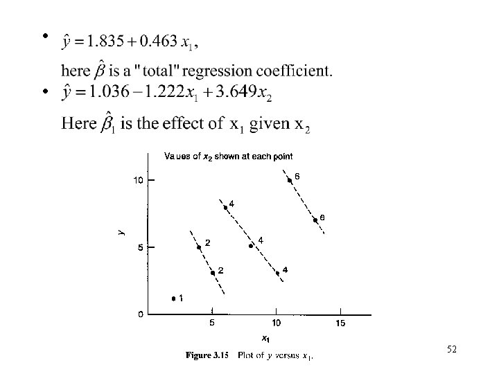
• For reason 1: 50

• Although it is possible to decrease the variance of the regression coefficients by increase the range of the x’s, it may not be desirable to spread the levels of the regressors out too far: – The true response function may be nonlinear. – Impractical or impossible. • For reason 2: 51

• Fore reason 3: Multicollinearity inflates the variances of the coefficients, and this increases the probability that one or more regression coefficients will have the wrong sign. • Different computer programs handle round-off or truncation problems in different ways, and some programs are more effective than the others in this regard. 53