3 1 Schrdinger Equation Postulate 6 Schrdinger Equation

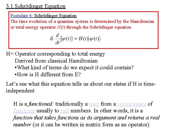
3. 1 Schrödinger Equation Postulate 6: Schrödinger Equation The time evolution of a quantum system is determined by the Hamiltonian or total energy operator H(t) through the Schrödinger equation H= Operator corresponding to total energy Derived from classical Hamiltonian • What kind of terms do we expect it could contain? • How is H different from E? Let’s see what this equation tells us about our states if H is timeindependent H is a functional: traditionally a map from a vector space of functions usually to real numbers. In other words, it is a function that takes functions as its argument and returns a real number (or it can be written in matrix form as an operator)

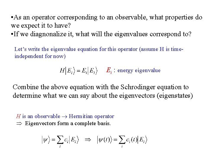
• As an operator corresponding to an observable, what properties do we expect it to have? • If we diagnonalize it, what will the eigenvalues correspond to? Let’s write the eigenvalue equation for this operator (assume H is timeindependent for now) Ei : energy eigenvalue Combine the above equation with the Schrodinger equation to determine what we can say about the eigenvectors (eigenstates) H is an observable Hermitian operator Eigenvectors form a complete basis.

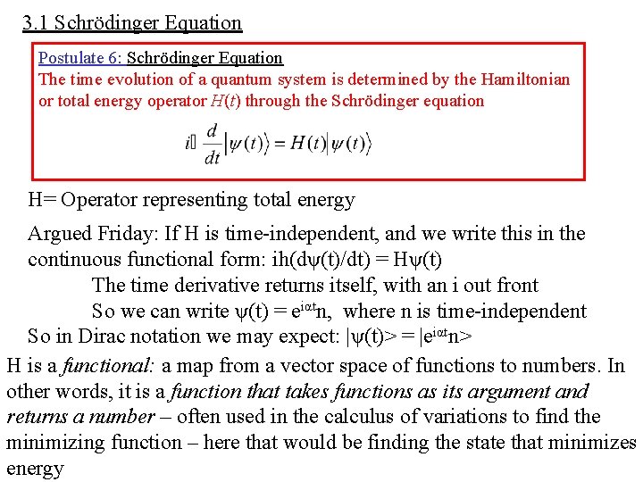
3. 1 Schrödinger Equation Postulate 6: Schrödinger Equation The time evolution of a quantum system is determined by the Hamiltonian or total energy operator H(t) through the Schrödinger equation H= Operator representing total energy Argued Friday: If H is time-independent, and we write this in the continuous functional form: ih(dψ(t)/dt) = Hψ(t) The time derivative returns itself, with an i out front So we can write ψ(t) = eiαtn, where n is time-independent So in Dirac notation we may expect: |ψ(t)> = |eiαtn> H is a functional: a map from a vector space of functions to numbers. In other words, it is a function that takes functions as its argument and returns a number – often used in the calculus of variations to find the minimizing function – here that would be finding the state that minimizes energy

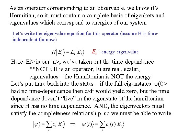
As an operator corresponding to an observable, we know it’s Hermitian, so it must contain a complete basis of eigenkets and eigenvalues which correspond to energies of our system Let’s write the eigenvalue equation for this operator (assume H is timeindependent for now) Ei : energy eigenvalue Here |Ei> is our |n>, we’ve taken out the time-dependence **NOTE H is an operator, Ei are real, scalar, eigenvalues – the Hamiltonian is NOT the energy! Let’s put time back into the states – if the full eigenstates |ψ(t)> had no time-dependence then d/dt would yield zero, but the time dependence doesn’t “live” in the eigenstate of the hamiltonian since H has no time dependence. AND, the eigenvectors must satisfy the completeness relationship, so we must be able to write:

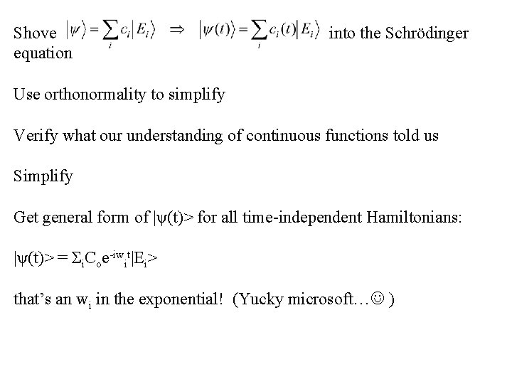
Shove equation into the Schrödinger Use orthonormality to simplify Verify what our understanding of continuous functions told us Simplify Get general form of |ψ(t)> for all time-independent Hamiltonians: |ψ(t)> = Σi. Coe-iwit|Ei> that’s an wi in the exponential! (Yucky microsoft… )

What will happen if our system starts in one particular energy eigenstate at t=0, say |E 2>, then we watch it for some time t – how do we write the state at time t? • How will the probability of finding the state with energy E 2 (or any energy) after time t differ from at time t=0? • How will the probabilities associated with any observations of this state after time t differ from at t=0? What name might you give such an initial “pure” state to explain how it behaves with time?

If our initial state at t=0 is a|E 1> + b|E 2>, what will be our state after some time t? • How will the probability of finding the state with energy E 2 (or any energy) after time t differ from at time t=0? • How will the probabilities associated with any observations of this state after time t differ from at t=0?

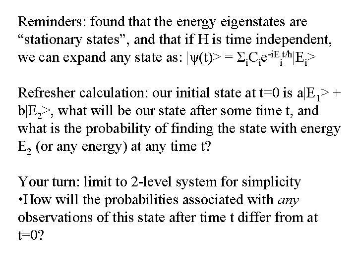
Reminders: found that the energy eigenstates are “stationary states”, and that if H is time independent, we can expand any state as: |ψ(t)> = Σi. Cie-i. Eit/ħ|Ei> Refresher calculation: our initial state at t=0 is a|E 1> + b|E 2>, what will be our state after some time t, and what is the probability of finding the state with energy E 2 (or any energy) at any time t? Your turn: limit to 2 -level system for simplicity • How will the probabilities associated with any observations of this state after time t differ from at t=0?

Energy eigenstates • Regardless of our initial energy eigenstate, the probability of observing the energy of the state does not change with time (that’s because our Hamiltonian, which represents total energy, is time independent!) • (This is true for any observable that commutes with H as well – since commuting observables share eigenstates) • However, if we are considering a general observable, our probability will oscillate with time! • angular frequency of the “time evolution” = Bohr Frequency ω12 = E 2 -E 1/ħ

Measurement of some other observable A – say position, momentum, or spin!! (1) If [A, H ] = 0, then observations won’t change with time – “stationary states” since A and H must share eigenstates (2) If [A, H ] 0, then observations will oscillate with time Look at example of time evolution of square well states using the Ph. ET simulation (http: //phet. colorado. edu) Explain what you observe in terms of our new understanding of “time evolution” of quantum states

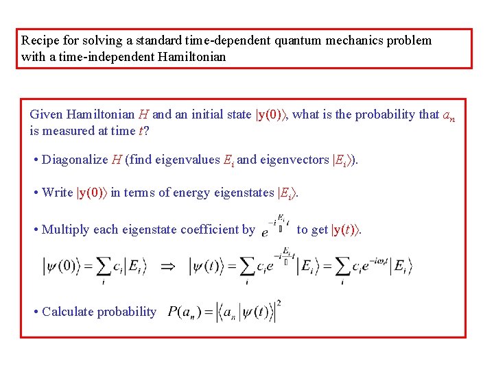
Recipe for solving a standard time-dependent quantum mechanics problem with a time-independent Hamiltonian Given Hamiltonian H and an initial state |y(0) , what is the probability that an is measured at time t? • Diagonalize H (find eigenvalues Ei and eigenvectors |Ei ). • Write |y(0) in terms of energy eigenstates |Ei. • Multiply each eigenstate coefficient by • Calculate probability to get |y(t).

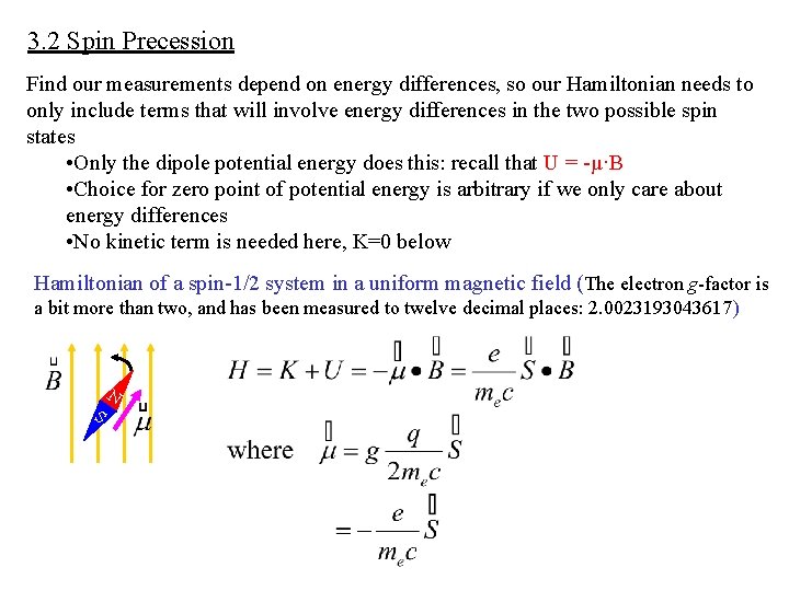
3. 2 Spin Precession Find our measurements depend on energy differences, so our Hamiltonian needs to only include terms that will involve energy differences in the two possible spin states • Only the dipole potential energy does this: recall that U = -μ·B • Choice for zero point of potential energy is arbitrary if we only care about energy differences • No kinetic term is needed here, K=0 below Hamiltonian of a spin-1/2 system in a uniform magnetic field (The electron g-factor is a bit more than two, and has been measured to twelve decimal places: 2. 0023193043617) N S

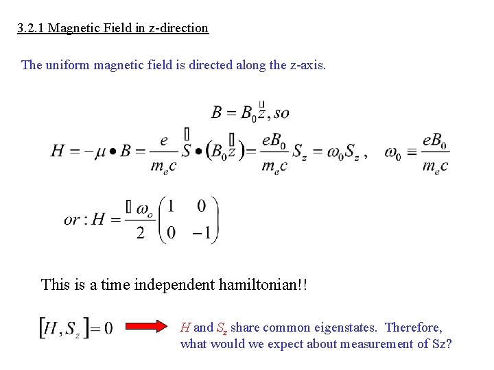
3. 2. 1 Magnetic Field in z-direction The uniform magnetic field is directed along the z-axis. This is a time independent hamiltonian!! H and Sz share common eigenstates. Therefore, what would we expect about measurement of Sz?

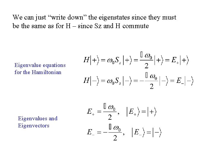
We can just “write down” the eigenstates since they must be the same as for H – since Sz and H commute Eigenvalue equations for the Hamiltonian Eigenvalues and Eigenvectors

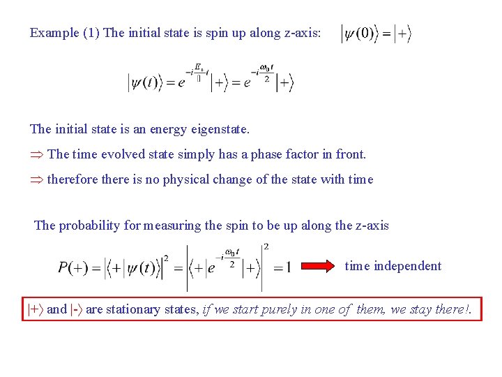
Example (1) The initial state is spin up along z-axis: The initial state is an energy eigenstate. The time evolved state simply has a phase factor in front. therefore there is no physical change of the state with time The probability for measuring the spin to be up along the z-axis time independent |+ and |- are stationary states, if we start purely in one of them, we stay there!.

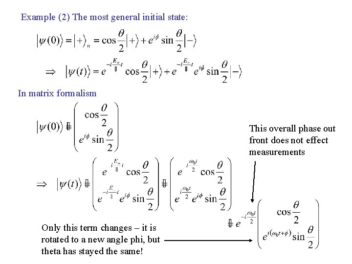
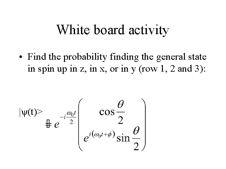
Example (2) The most general initial state: In matrix formalism This overall phase out front does not effect measurements Only this term changes – it is rotated to a new angle phi, but theta has stayed the same!

White board activity • Find the probability finding the general state in spin up in z, in x, or in y (row 1, 2 and 3): |ψ(t)>

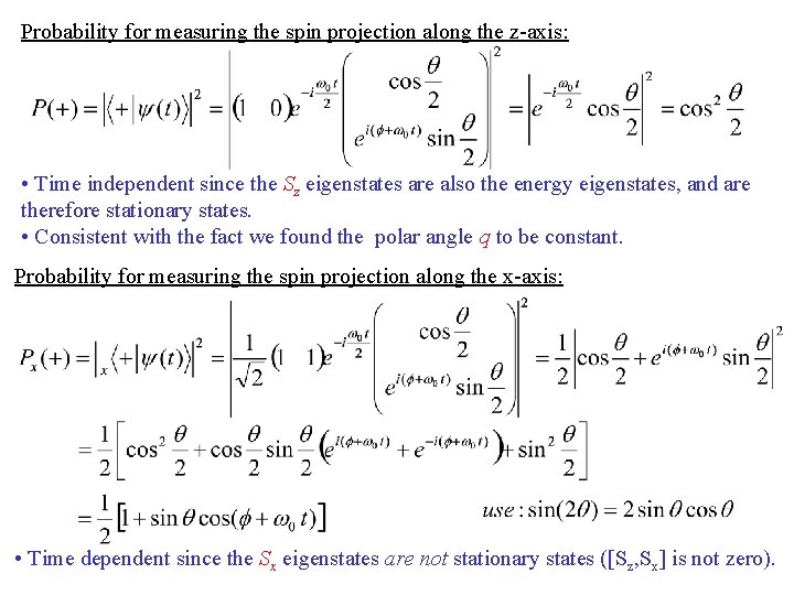
Probability for measuring the spin projection along the z-axis: • Time independent since the Sz eigenstates are also the energy eigenstates, and are therefore stationary states. • Consistent with the fact we found the polar angle q to be constant. Probability for measuring the spin projection along the x-axis: • Time dependent since the Sx eigenstates are not stationary states ([Sz, Sx] is not zero).

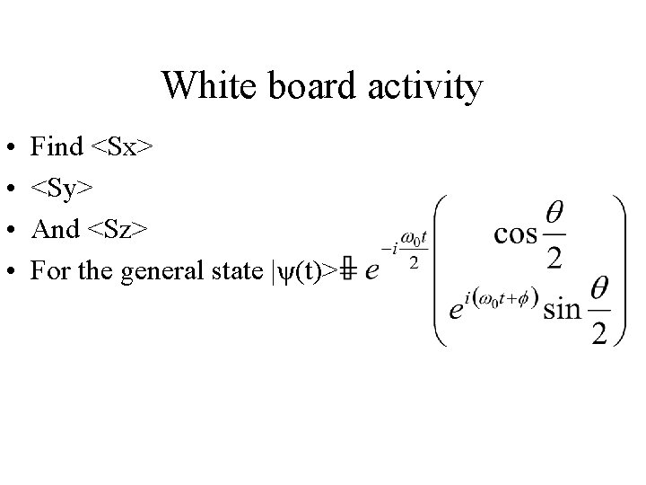
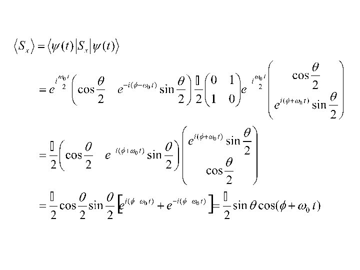
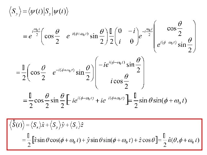
White board activity • • Find <Sx> <Sy> And <Sz> For the general state |ψ(t)>

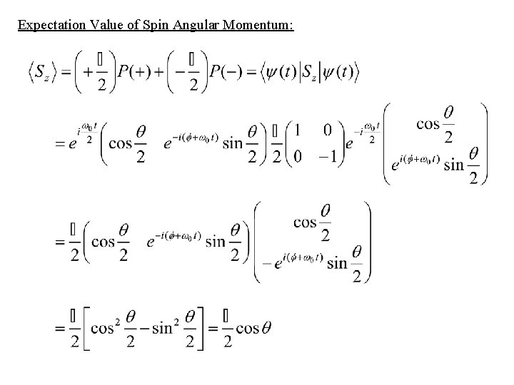
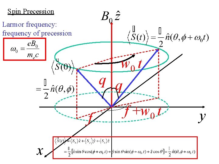
Expectation Value of Spin Angular Momentum:

Spin Precession Larmor frequency: frequency of precession w 0 t q q f x f +w 0 t y

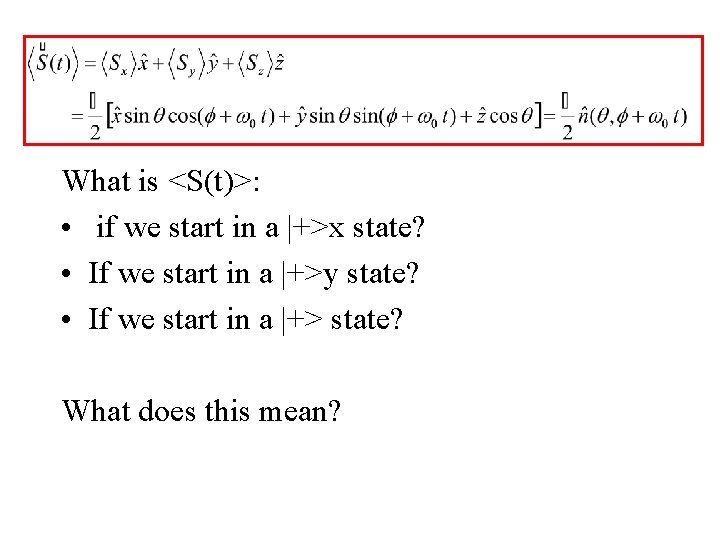
What is <S(t)>: • if we start in a |+>x state? • If we start in a |+>y state? • If we start in a |+> state? What does this mean?

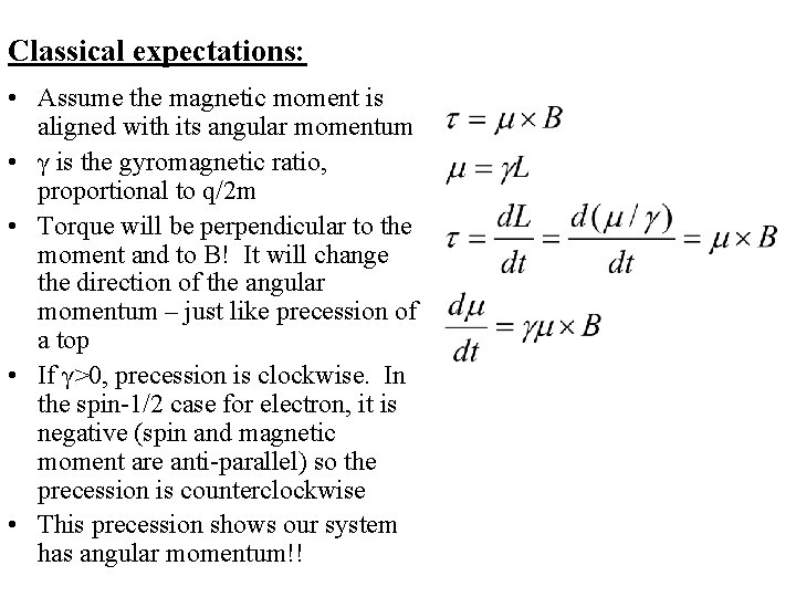
Classical expectations: • Assume the magnetic moment is aligned with its angular momentum • γ is the gyromagnetic ratio, proportional to q/2 m • Torque will be perpendicular to the moment and to B! It will change the direction of the angular momentum – just like precession of a top • If γ>0, precession is clockwise. In the spin-1/2 case for electron, it is negative (spin and magnetic moment are anti-parallel) so the precession is counterclockwise • This precession shows our system has angular momentum!!

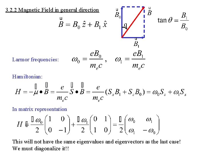
3. 2. 2 Magnetic Field in general direction q Larmor frequencies: Hamiltonian: In matrix representation This will not have the same eigenvalues and eigenvectors as the last case! We must diagonalize it!!

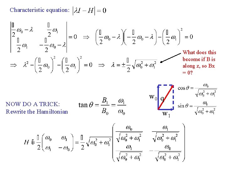
Characteristic equation: What does this become if B is along z, so Bx = 0? NOW DO A TRICK: Rewrite the Hamiltonian w 0 q w 1

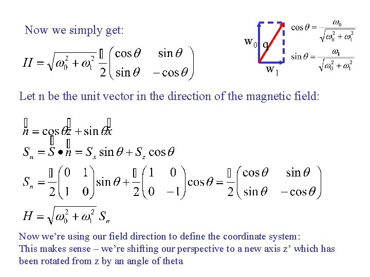
Now we simply get: w 0 q w 1 Let n be the unit vector in the direction of the magnetic field: Now we’re using our field direction to define the coordinate system: This makes sense – we’re shifting our perspective to a new axis z’ which has been rotated from z by an angle of theta

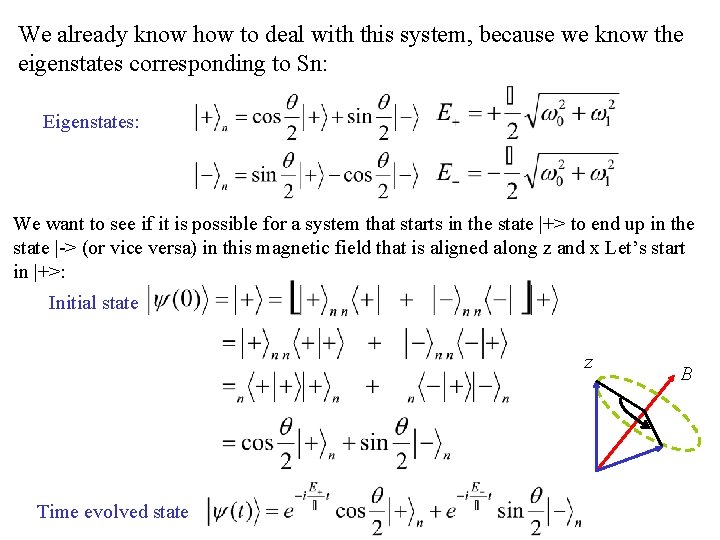
We already know how to deal with this system, because we know the eigenstates corresponding to Sn: Eigenstates: We want to see if it is possible for a system that starts in the state |+> to end up in the state |-> (or vice versa) in this magnetic field that is aligned along z and x Let’s start in |+>: Initial state z Time evolved state B

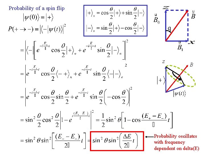
Probability of a spin flip q z B Probability oscillates with frequency dependent on delta(E)

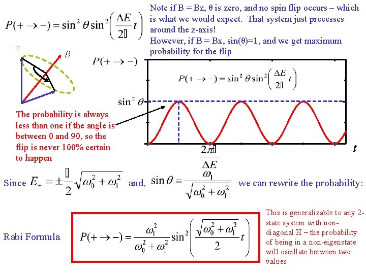
z Note if B = Bz, θ is zero, and no spin flip occurs – which is what we would expect. That system just precesses around the z-axis! However, if B = Bx, sin(θ)=1, and we get maximum probability for the flip B The probability is always less than one if the angle is between 0 and 90, so the flip is never 100% certain to happen Since Rabi Formula t and, we can rewrite the probability: This is generalizable to any 2 state system with nondiagonal H – the probability of being in a non-eigenstate will oscillate between two values

Understanding “spin space” • You know 3 -d space isn’t the same as our spin space – Evidence: the “length” of the spin vector is longer than we can ever measure – more or less meaning we can’t align real space perfectly parallel to spin space – We must be careful when interpreting any physical picture of spin! (they are all “unsatisfactory” and can be misleading if this fact is forgotten)

In words of QM theorist at Los Alamos: • Quantum objects are like what classical things look to someone with bad eyesight: a quantum spin half object is like a cylinder with one red end and one green end looked at by someone with such bad eyesight that it looks more like a fuzzy sphere. So, the red side basically points out a hemisphere towards which it points. The abstract vector space is a space in which every classical hemisphere (or smaller solid angle for larger spin value) is a point. You can naively associate the central direction as the classical vector, as long as you remember the irreducible fuzzyness. • the superposition principle that lies behind the construction of the state vector space is the most difficult bit in QM. The hemisphere picture works somewhat but is not very clean… I know that almost everybody involved in understanding why quantum computation is faster than classical computation for some problems would like to understand this. It is also at the heart of most controversies about interpretation of quantum mechanics. So, if textbooks don't have a good picture, its because the author doesn't.

Some possibly interesting papers • “Delirium Quantum: Or where I will take quantum mechanics if it will let me” by Christopher Fuchs at Bell Labs, 2009 • http: //arxiv. org/PS_cache/arxiv/pdf/0906. 1968 v 1. pdf • “Nonlinear Quantum Mechanics, the Superposition Principle, and the Quantum Measurement Problem” by Kinjalk Lochan and T. P. Singh at. Tata Institute, 2009 • http: //arxiv. org/PS_cache/arxiv/pdf/0912. 2845 v 2. pdf

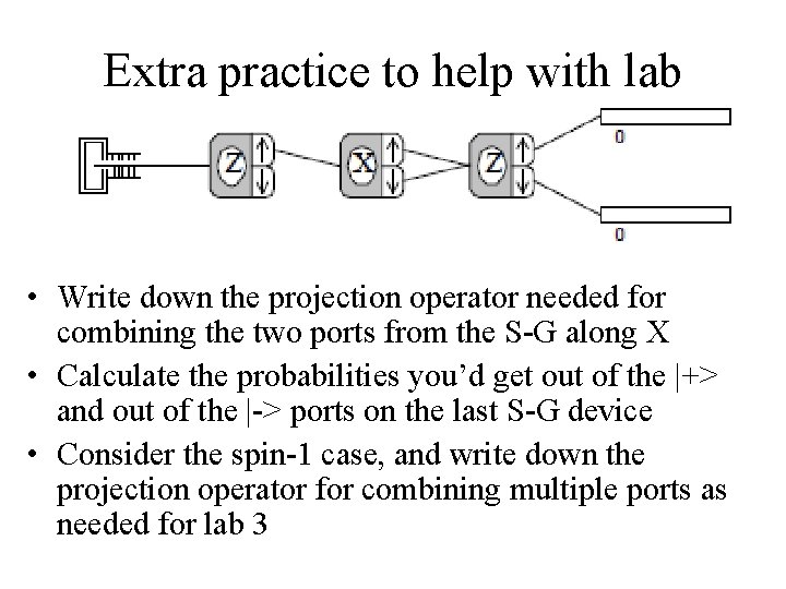
Extra practice to help with lab • Write down the projection operator needed for combining the two ports from the S-G along X • Calculate the probabilities you’d get out of the |+> and out of the |-> ports on the last S-G device • Consider the spin-1 case, and write down the projection operator for combining multiple ports as needed for lab 3

Neutrino Oscillations • What are neutrinos? • http: //www. particleadventure. org/index. html • Tau neutrino discovered at Fermilab in 2000 – strong evidence for 3 “generations” of standard model • 1998 was first report of evidence for neutrino oscillation (at Super-K in Japan) • “missing solar neutrinos” in 2001 – realized to be due to oscillations – Proton mass is ~1 Ge. V – Electron mass ~1 Me. V – Neutrino mass <1 e. V!

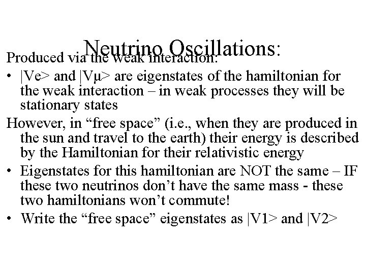
Oscillations: Produced via. Neutrino the weak interaction: • |Ve> and |Vμ> are eigenstates of the hamiltonian for the weak interaction – in weak processes they will be stationary states However, in “free space” (i. e. , when they are produced in the sun and travel to the earth) their energy is described by the Hamiltonian for their relativistic energy • Eigenstates for this hamiltonian are NOT the same – IF these two neutrinos don’t have the same mass - these two hamiltonians won’t commute! • Write the “free space” eigenstates as |V 1> and |V 2>

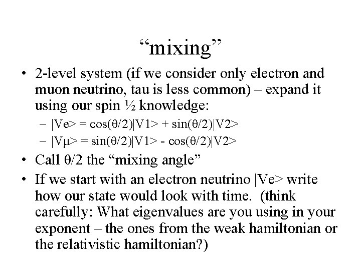
“mixing” • 2 -level system (if we consider only electron and muon neutrino, tau is less common) – expand it using our spin ½ knowledge: – |Ve> = cos(θ/2)|V 1> + sin(θ/2)|V 2> – |Vμ> = sin(θ/2)|V 1> - cos(θ/2)|V 2> • Call θ/2 the “mixing angle” • If we start with an electron neutrino |Ve> write how our state would look with time. (think carefully: What eigenvalues are you using in your exponent – the ones from the weak hamiltonian or the relativistic hamiltonian? )

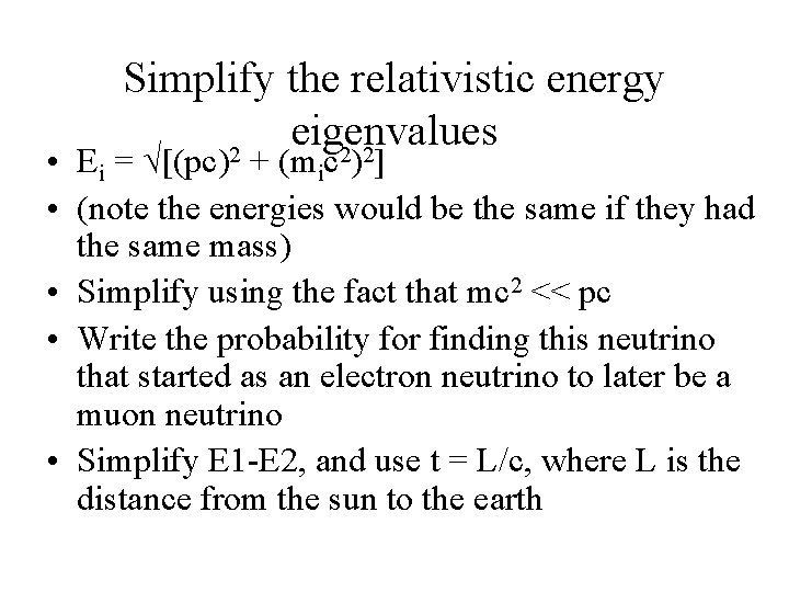
Simplify the relativistic energy eigenvalues 2 2 2 • Ei = √[(pc) + (mic ) ] • (note the energies would be the same if they had the same mass) • Simplify using the fact that mc 2 << pc • Write the probability for finding this neutrino that started as an electron neutrino to later be a muon neutrino • Simplify E 1 -E 2, and use t = L/c, where L is the distance from the sun to the earth

“Super-K” (Kamiokande) • http: //en. wikipedia. org/wiki/Super-Kamiokande

Why are neutrinos massive? • In Standard Model, fermions have mass because of interactions with Higgs field (Higgs boson), but this can’t explain neutrino mass • Mass of neutrino is at least 500, 000 times smaller than the mass of an electron, so any correction to standard model wouldn’t explain why the mass is SO small • This remains unexplained • http: //en. wikipedia. org/wiki/Neutrino_oscillations

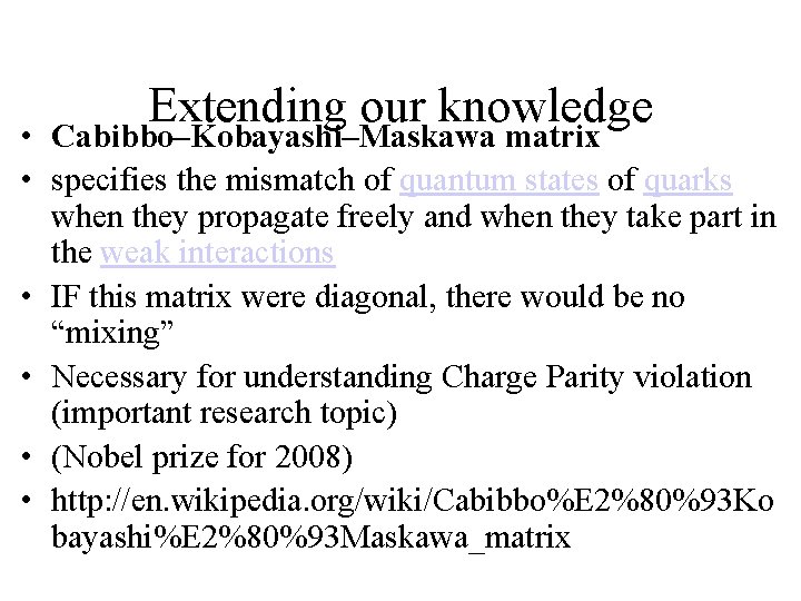
Extending our knowledge • Cabibbo–Kobayashi–Maskawa matrix • specifies the mismatch of quantum states of quarks when they propagate freely and when they take part in the weak interactions • IF this matrix were diagonal, there would be no “mixing” • Necessary for understanding Charge Parity violation (important research topic) • (Nobel prize for 2008) • http: //en. wikipedia. org/wiki/Cabibbo%E 2%80%93 Ko bayashi%E 2%80%93 Maskawa_matrix