3 1 Clustering Finding a good clustering of

3. 1 Clustering Finding a good clustering of the points is a fundamental issue in computing a representative simplicial complex. Mapper does not place any conditions on the clustering algorithm. Thus any domain-specific clustering algorithm can be used.

We implemented a clustering algorithm for testing the ideas presented here. The desired characteristics of the clustering were: 1. Take the inter-point distance matrix (D∈RN×N) as an input. We did not want to be restricted to data in Euclidean Space. 2. Do not require specifying the number of clusters beforehand.

We have implemented an algorithm based on singlelinkage clustering [Joh 67], [JD 88]. This algorithm returns a vector C ∈ RN− 1 which holds the length of the edge which was added to reduce the number of clusters by one at each step in the algorithm. Now, to find the number of clusters we use the edge length at which each cluster was merged.

The heuristic is that the inter-point distance within each cluster would be smaller than the distance between clusters, so shorter edges are required to connect points within each cluster, but relatively longer edges are required to merge the clusters.

If we look at the histogram of edge lengths in C, it is observed experimentally, that shorter edges which connect points within each cluster have a relatively smooth distribution and the edges which are required to merge the clusters are disjoint from this in the histogram.

If we determine the histogram of C using k intervals, then we expect to find a set of empty interval(s) after which the edges which are required to merge the clusters appear. If we allow all edges of length shorter than the length at which we observe the empty interval in the histogram, then we can recover a clustering of the data.

Increasing k will increase the number of clusters we observe and decreasing k will reduce it. Although this heuristic has worked well for many datasets that we have tried, it suffers from the following limitations: (1) If the clusters have very different densities, it will tend to pick out clusters of high density only. (2) It is possible to construct examples where the clusters are distributed in such a way such that we recover the incorrect clustering. Due to such limitations, this part of the procedure is open to exploration and change in the future.

3. 2. Higher Dimensional Parameter Spaces Using a single function as a filter we get as output a complex in which the highest dimension of simplices is 1 (edges in a graph). Qualitatively, the only information we get out of this is the number of components, the number of loops and knowledge about structure of the component flares etc. ).

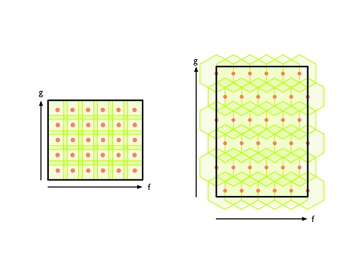
To get information about higher dimensional voids in the data one would need to build a higher dimensional complex using more functions on the data. In general, the Mapper construction requires as input: (a) A Parameter space defined by the functions and (b) a covering of this space. Note that any covering of the parameter space may be used. As an example of the parameter space S 1, consider a parameter space defined by two functions f and g which are related such that f 2+g 2 = 1. A very simple covering for such a space is generated by considering overlapping angular intervals.

An algorithm for building a reduced simplicial complex is: 1. For each i, j, select all data points for which the function values of f 1 and f 2 lie within Ai, j. Find a clustering of points for this set and consider each cluster to represent a 0 dimensional simplex (referred to as a vertex in this algorithm). Also, maintain a list of vertices for each Ai, j and a set of indices of the data points (the cluster members) associated with each vertex. 2. For all vertices in the sets {Ai, j , Ai+1, j , Ai, j+1, Ai+1, j+1}, if the intersection of the cluster associated with the vertices is non-empty then add a 1 -simplex (referred to as an edge in this algorithm). 3. Whenever clusters corresponding to any three vertices have non empty intersection, add a corresponding 2 simplex (referred to as a triangle in this algorithm) with the three vertices forming its vertex set. 4. Whenever clusters corresponding to any four vertices have non-empty intersection, add a 3 simplex (referred to as tetrahedron in this algorithm) with the four vertices forming its vertex set. It is very easy to extend Mapper to the parameter space RMin a similar fashion.

Example 3. 4 Consider the unit sphere in R 3. Refer to Figure 3. The functions are f 1(x) = x 3 and f 2(x) = x 1, where x = (x 1, x 2, x 3). As intervals in the range of f 1 and f 2 are scanned, we select points from the dataset whose function values lie in both the intervals and then perform clustering. In case of a sphere, clearly only three possibilities exist: 1. The intersection is empty, and we get no clusters. 2. The intersection contains only one cluster. 3. The intersection contains two clusters. After finding clusters for the covering, we form higher dimensional simplices as described above. We then used the homology detection software PLEX ( [Pd. S]) to analyze the resulting complex and to verify that this procedure recovers the correct Betti numbers: b 0 = 1, b 1 = 0, b 2 = 1.

Figure 3: Refer to Example 3. 4 for details. Let the filtering functions be f 1(x) = x 3, f 2(x) = x 1, where xi is the ith coordinate. The top two images just show the contours of the function f 1 and f 2 respectively. The three images in the middle row illustrate the possible clusterings as the ranges of f 1 and f 2 are scanned. The image in the bottom row shows the number of clusters as each region in the range( f 1)×range( f 2) is considered.

5. Sample Applications In this section, we discuss a few applications of the Mapper algorithm using our implementation. Our aim is to demonstrate the usefulness of reducing a point cloud to a much smaller simplicial complex in synthetic examples and some real data sets. We have implemented the Mapper algorithm for computing and visualizing a representative graph (derived using one function on the data) and the algorithm for computing a higher order complex using multiple functions on the data. Our implementation is in MATLAB and utilizes Graph. Viz for visualization of the reduced graphs

Different type of hierarchical clustering What is the distance between 2 clusters? http: //en. wikipedia. org/wiki/File: Hiera rchical_clustering_simple_diagram. svg http: //www. multid. se/genex/hs 515. htm

http: //statweb. stanford. edu/~tibs/Elem. Stat. Learn/ The Elements of Statistical Learning (2 nd edition) Hastie, Tibshirani and Friedman

http: //scikit-learn. org/stable/auto_examples/cluster/plot_cluster_comparison. html